Design Information Bulletin No 87-01 Appendices

Table of Contents

Appendix A: Hydraulic Model Calibration

Appendix B: Sample Hydraulic Models

Appendix C: Sample Hybrid Revetment Plan Sheets & Design Cross Sections

Appendix D: Gravel Filter Nonstandard Special Provision

Appendix A - Hydraulic Model Calibration

Simple Calibration Using Field Measured Flow-Depth and Velocity

The following is a basic procedure for calibrating a HEC-RAS model with field measured stream depth and velocity of flowing water at a single location. The gathering of field data is recommended at several locations when possible.

Step1: At a stream with flowing water, measure flow-depth and corresponding velocity at a known stream station.

Step 2: Using MicroStation or AutoCAD, plot the uniform (constant) water surface on the existing cross section station based on the measured flow-depth.

Step 3: Use MicroStation or AutoCAD tools to measure the wetted area of the cross section based on field measured flow-depth.

Step 4: Calculate a volume flow rate (flow) using the continuity equation considering the field measured velocity and wetted area found in MicroStation or AutoCAD.

Q=vA

Q= volume flow rate (flow)

v= field measured velocity at specific flow-depth

A= wetted area based on field measured flow-depth

Step 5: Enter the calculated flow into HEC-RAS associated with the field measured flow-depth.

Step 6: In HEC-RAS, iteratively increase or decrease n-value at the specific stream station, and run HEC-RAS simulation until the HEC-RAS flow-depth matches the field measured flow-depth. The n-value used to match field flow-depth results can be considered for final pre-construction model use. It is good to have field measurements at a number of stream stations in order to find the most representative n-values.

Most likely, this calibration and roughness value refinement is only for the main channel considering the need for flowing water in the field. Typically, the floodplain overbanks receive flow much less frequently making it difficult to gather actual flow-depth and velocity in the field.

Simple Calibration Using Field Located Watermark

Roughness values can be refined by using watermarks from past storm flows found in the field, which aid in calibrating a HEC-RAS model. They can be used in the main channel or more commonly in the floodplain overbanks where flowing water occurs less frequently. This process of calibration requires more effort than the previous and is not as precise mainly because velocity cannot be measured in the field associated with a watermark opposed to flowing water.

The following is a basic process for calibrating a HEC-RAS model with a field located watermark at a single location. The gathering of field data is recommended at several locations when possible.

Step1: At a stream station, measure the vertical depth from the stream bed thalweg to the field watermark, which will be an assumed flow-depth.

Step2: Using MicroStation or AutoCAD, plot the uniform (constant) water surface on the existing cross section station based on the assumed flow-depth from the watermark.

Step 3: Use MicroStation or AutoCAD tools to measure the wetted area and wetted perimeter of the wetted cross section based on the assumed flow-depth from the watermark. If the watermark is within the floodplain overbank, separate wetted perimeters for the main channel and each overbank will need to be performed to calculate a composite n-value (see Step 4). These separate wetted perimeters would be in addition to the overall wetted perimeter of the entire wetted stream cross section.

Step 4: Since velocity is unknown, the continuity equation cannot be used as done above. Instead, Manning’s equation, solved for Q (flow), can be used to calculate an approximate flow rate corresponding to a field watermark, but will require an initial n-value to be determined and assumed for the cross section containing the watermark in order to calculate the approximate flow. This initial n-value will only be used to find a volume flow rate based on uniform flow theory associated with the watermark.

If the watermark is only contained in the main channel, the procedure to estimate a pre-construction main channel roughness value discussed in Section 6.1.2.1 can be used in Manning’s equation to calculate an approximate flow associated with the watermark.

Should the watermark be located within the floodplain overbanks, a composite n-value with consideration of the main channel and the overbanks must be determined to use in Manning’s equation (Section 6.1.2.1 can also be used to estimate floodplain overbank n-values). Each roughness value will be weighted by its wetted perimeter in the equation below for the calculation of a composite value.

n_c= (P_wLOB n_LOB + P_wMC n_MC + P_wROB n_ROB) P_wt^-1

P_wLOB= wetted perimeter of left overbank

n_LOB= estimated n-value of left overbank

P_wMC= wetted perimeter of main channel

n_MC= estimated n-value of main channel

P_wROB= wetted perimeter of right overbank

n_ROB= estimated n-value of right overbank

P_wt= sum of wetted perimeters

Step 5: After determination of an initial n-value, use Manning’s equation (based on uniform flow principle) to calculate an approximate flow associated with the field located watermark. In this calculation, use the wetted area and hydraulic radius based on the entire wetted cross section, determined from MicroStation or AutoCAD tools, as well as the slope of the stream approximated from existing cross sections.

Q= 1.49n_i^-1AR^2/3S^1/2

Q= approximate volume flow rate (flow)

n_i= initial (estimated) n-value

A= wetted area

R= hydraulic radius= A/P

P= wetted perimeter

S= stream bed slope

Step 6: Enter the calculated, approximate flow into HEC-RAS associated with the field watermark flow-depth.

Step 7: In HEC-RAS, iteratively increase or decrease n-value(s) at the specific stream station, and run HEC-RAS simulation until the HEC-RAS flow-depth matches the field measured watermark flow-depth.

As mentioned in Section 6.1.2, HEC-RAS provides solution using gradually varied flow in its analysis, which is more accurate than the uniform flow assumption used to approximate the volume flow rate corresponding to the watermark in Step 5.

If more than one roughness value (main channel, left overbank, right overbank) is being adjusted at the cross section, as in the case where the watermark is within the floodplain overbanks, many combinations of n-values exist that will yield the desired flow-depth. In other words, multiple combinations of roughness values exist that will produce the watermark flow-depth.

The n-value(s) used to match field flow-depth results can be considered for final pre-construction model use. It is good to have field measurements at a number of stream stations in order to find the most representative n-value(s).

Appendix B - Sample Hydraulic Models

Project Summary

Problem:

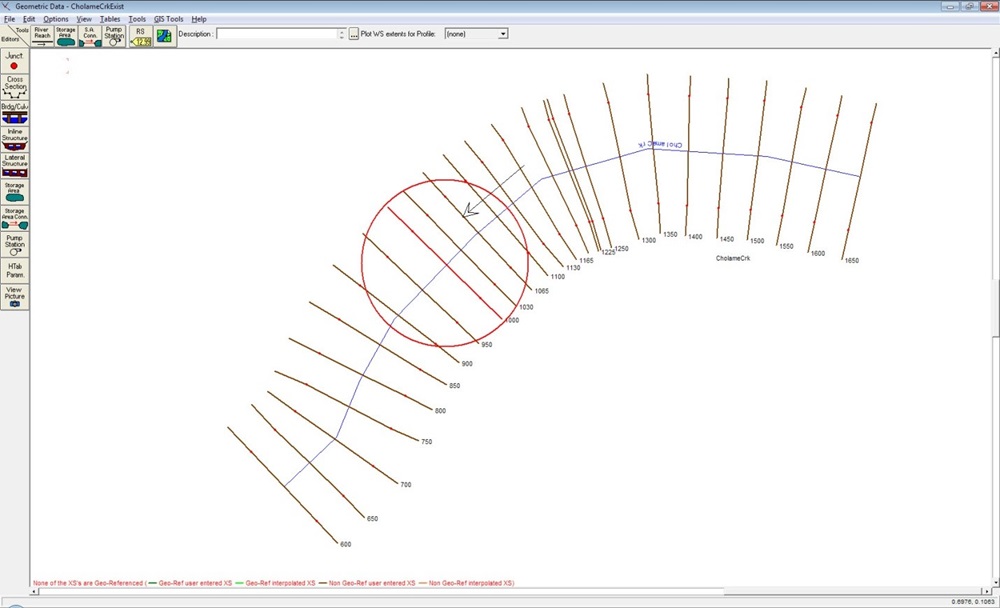
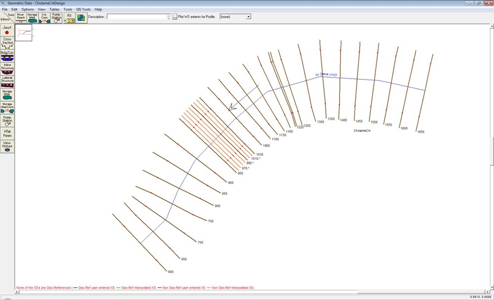
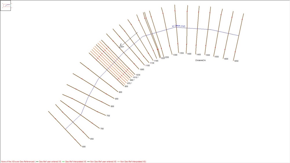
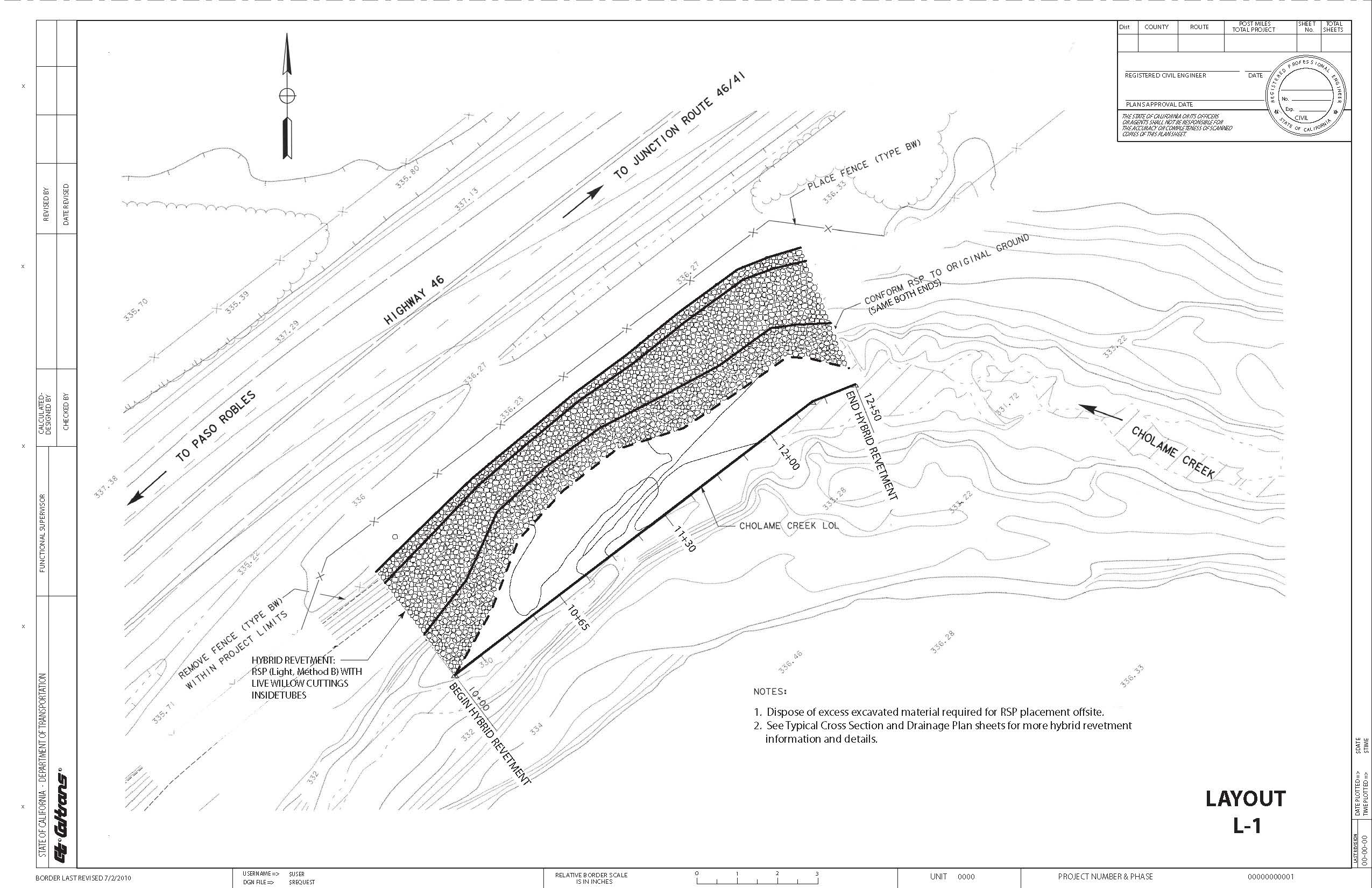
A portion of Cholame Creek, having a horizontal bend, runs parallel to Highway 46 and is subject to impinging flow. The left (outside) bank of the bend has been eroding over time and is in need of stabilization to control future scour and erosion.

Solution:

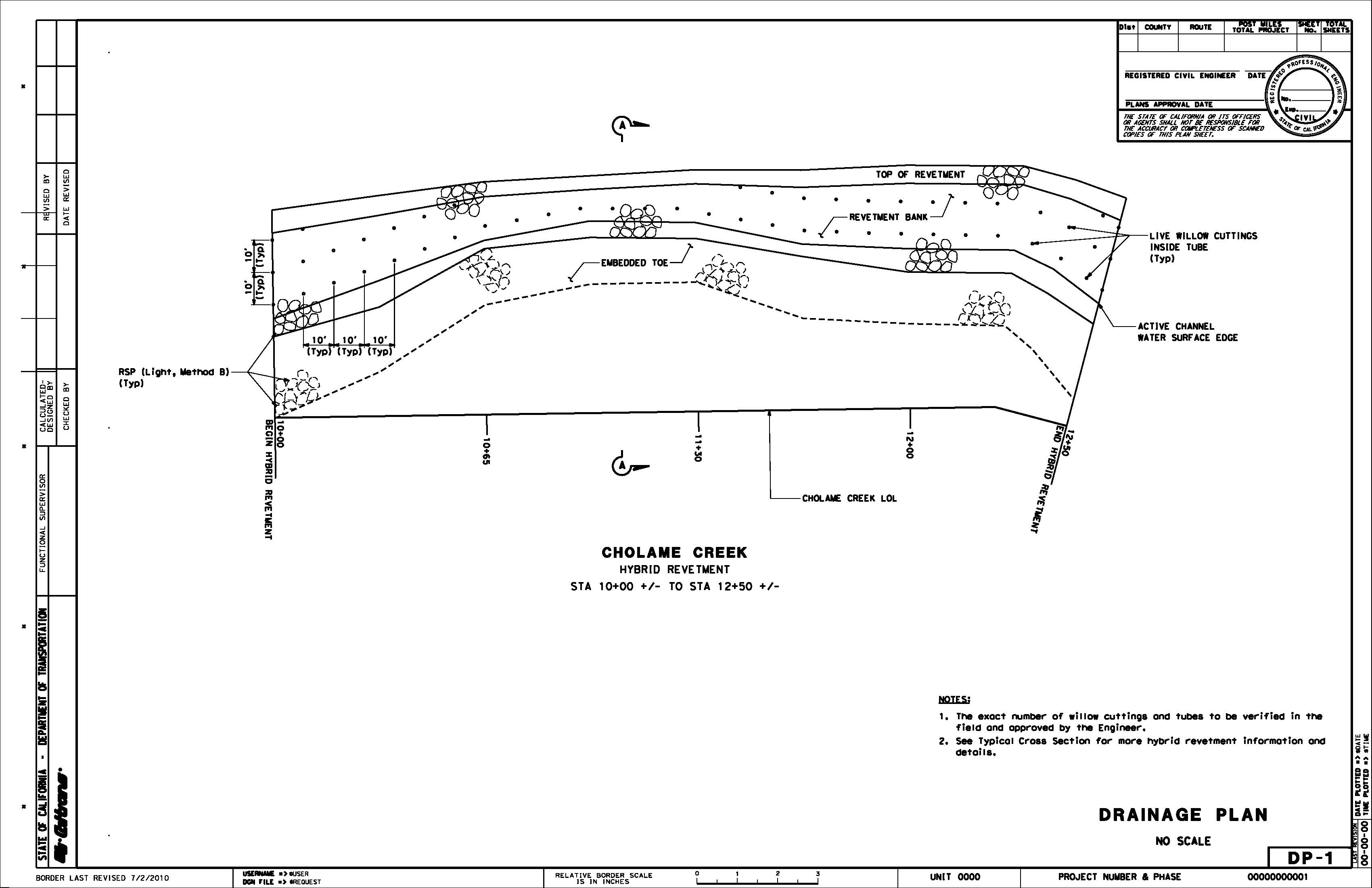
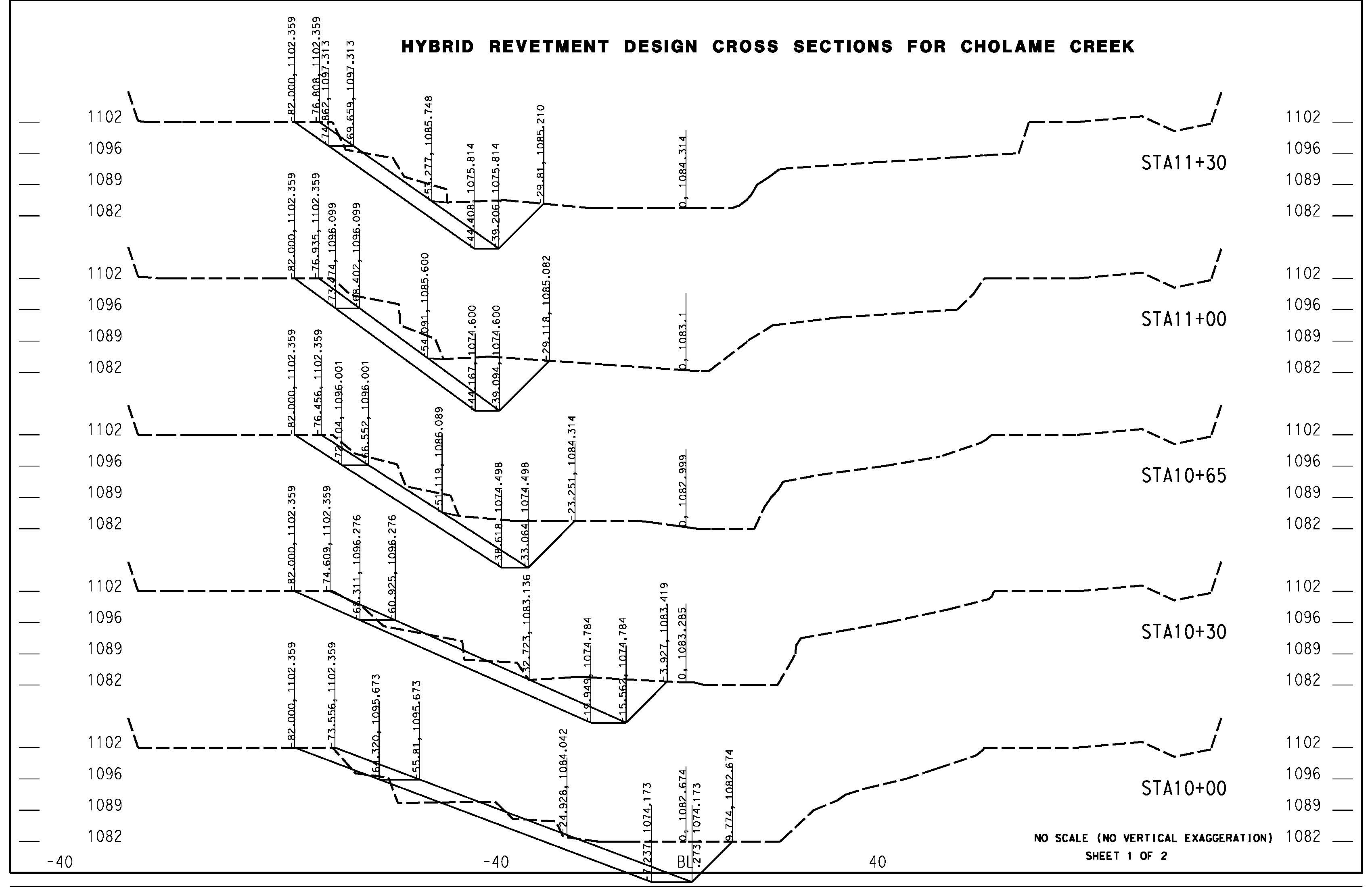
Construct a hybrid revetment having medium vegetation density to repair and stabilize left bank of main channel from STA 10+00 to STA 12+50.

Hydrolog:

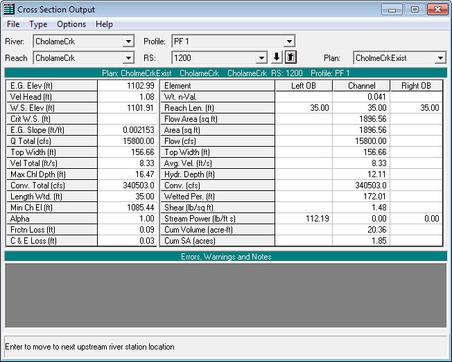
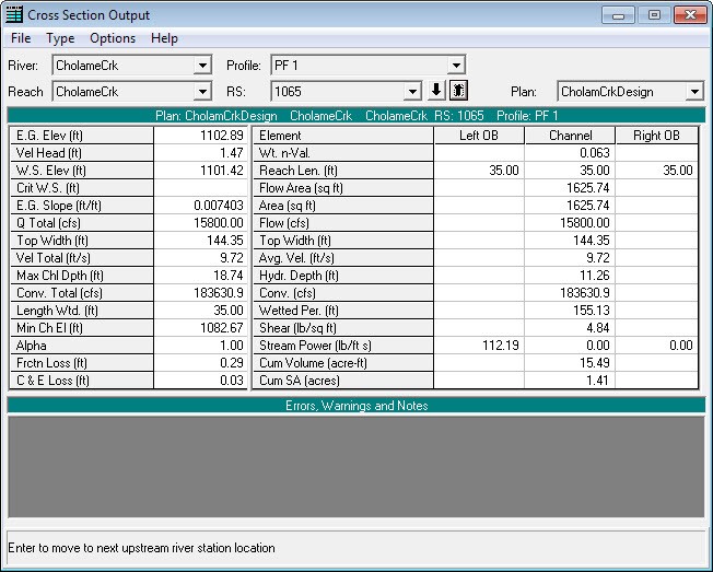
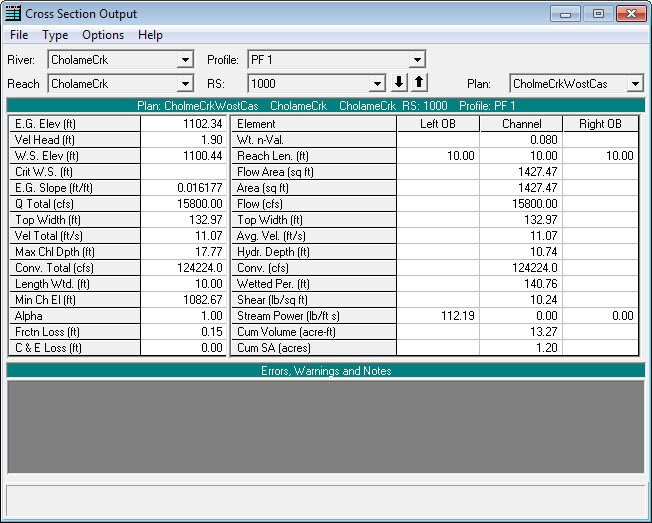
Q₅₀= 5,825 cubic feet/second (cfs) Q₁₀₀= 15,800 cfs

Hydraulics:

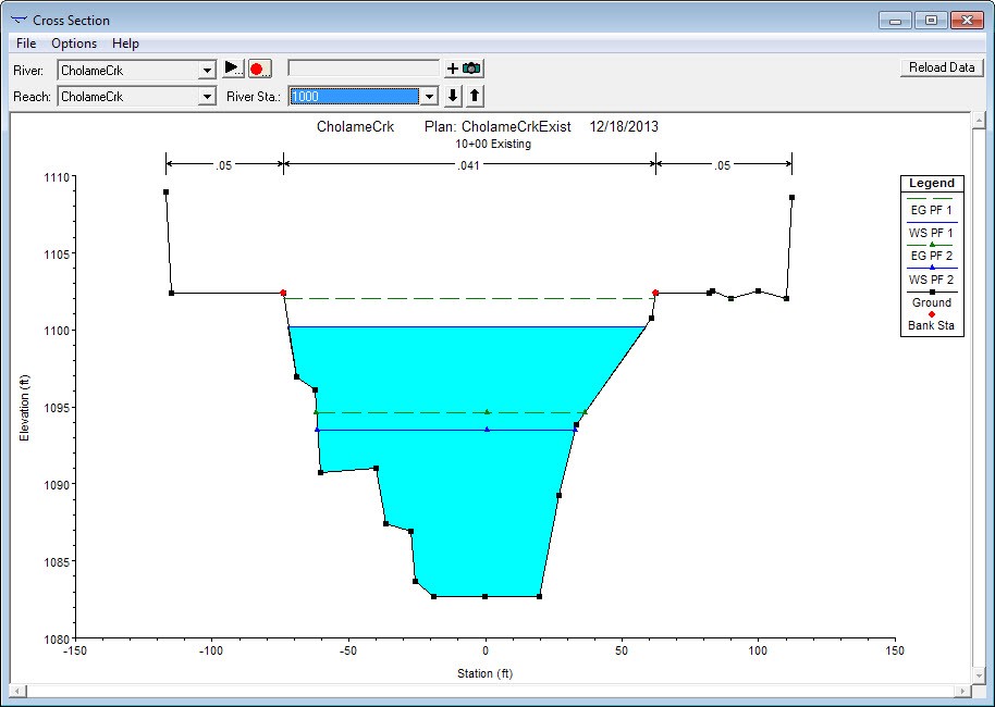
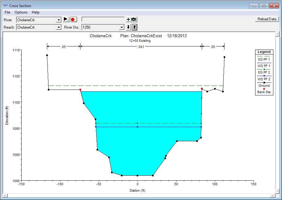
Pre-Construction Condition:

n= 0.050 (left & right overbanks)

n= 0.041 (main channel)

V₅₀₌ 9.2 feet/second (design velocity)

Flow-depth (d₅₀)= 11 feet (design high water)

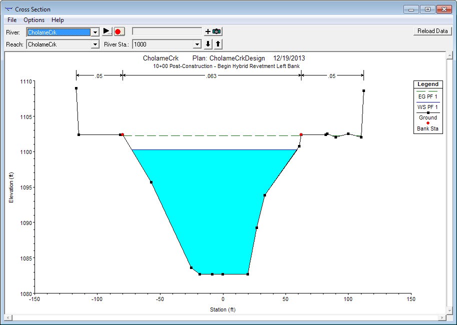
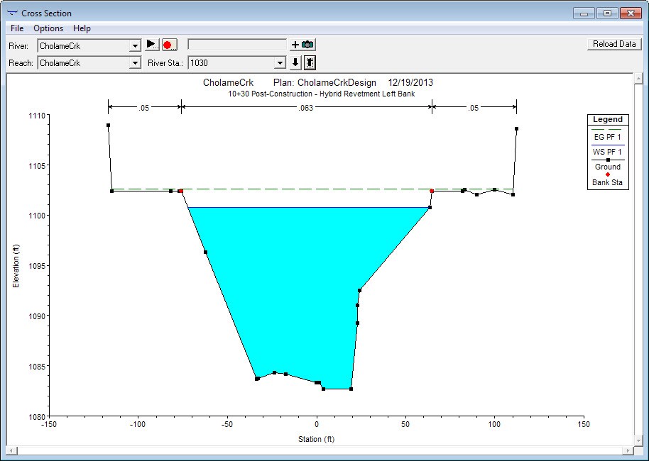
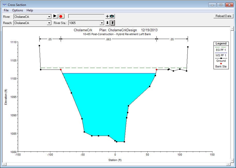
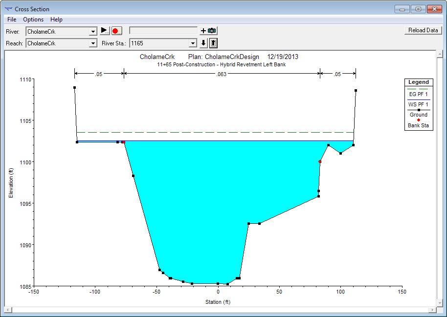
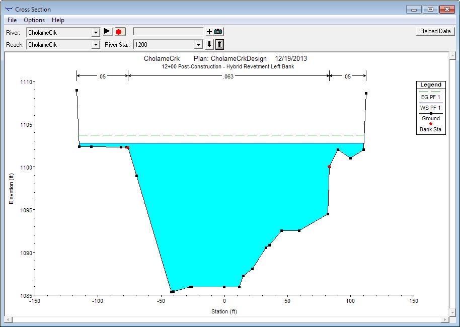
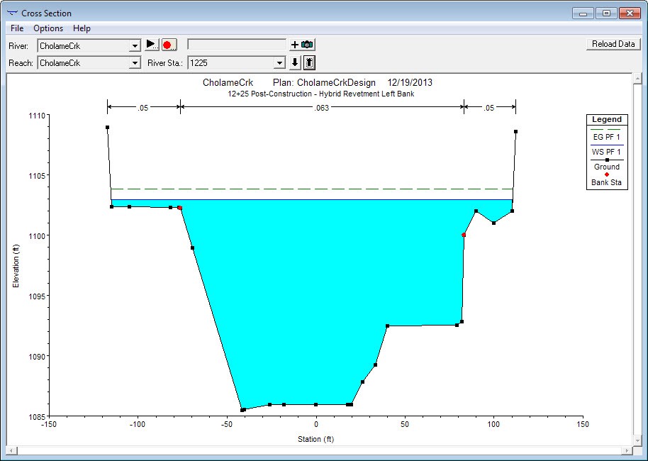
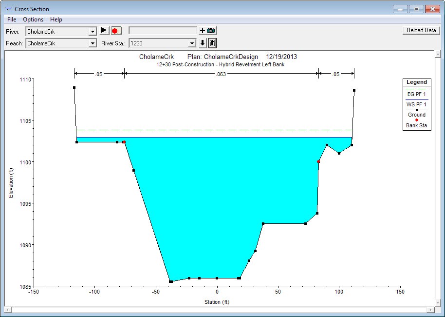
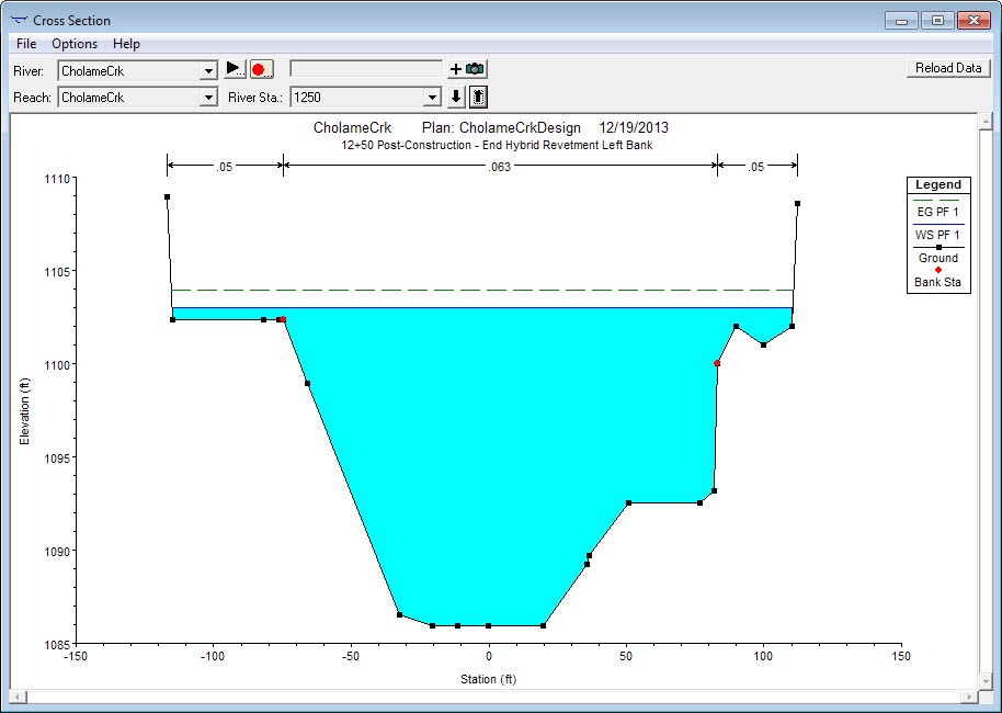
Post-Construction Condition:

n= 0.050 (left & right overbanks)

n= 0.063 (STA 10+00 to STA 12+50, main channel considering hybrid revetment with medium vegetation density)

n= 0.041 (main channel: upstream & downstream of hybrid revetment)

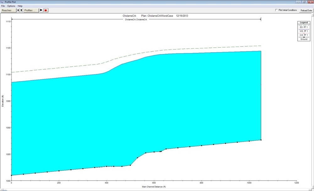
Worst-Case Condition:

n= 0.050 (left & right overbanks)

n= 0.080 (STA 10+00 to STA 12+50, main channel considering hybrid revetment with high vegetation density)

n= 0.041 (main channel: upstream & downstream of hybrid revetment)

Hybrid Revetment Design Information

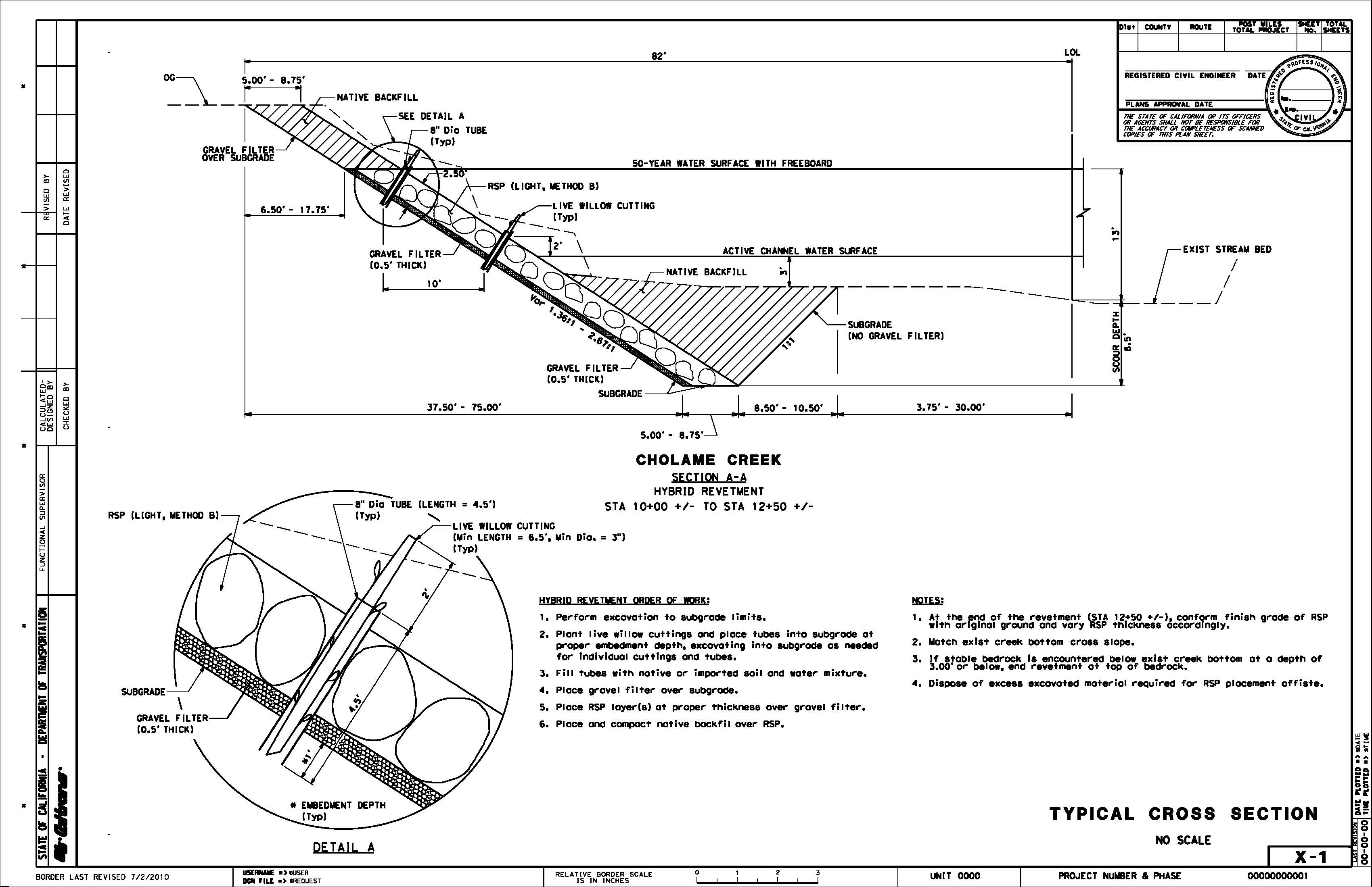
• Revetment Length= 250 feet
• Revetment Height= 11 feet (design high water) + 2 feet (freeboard)= 13 feet
• RSP Light (2.5 feet thick) underlain by gravel filter (0.5 feet thick)
• Medium Vegetation Density: willow cuttings planted every 10 feet longitudinally and laterally and perpendicular orientation with streambank

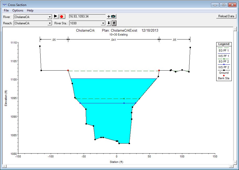
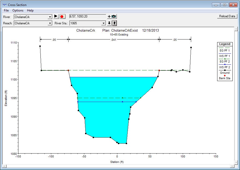
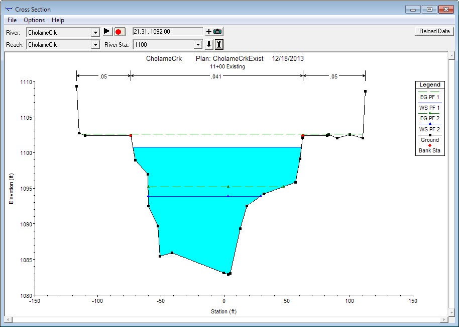
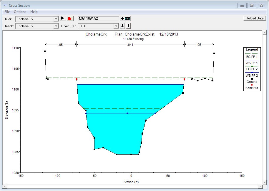
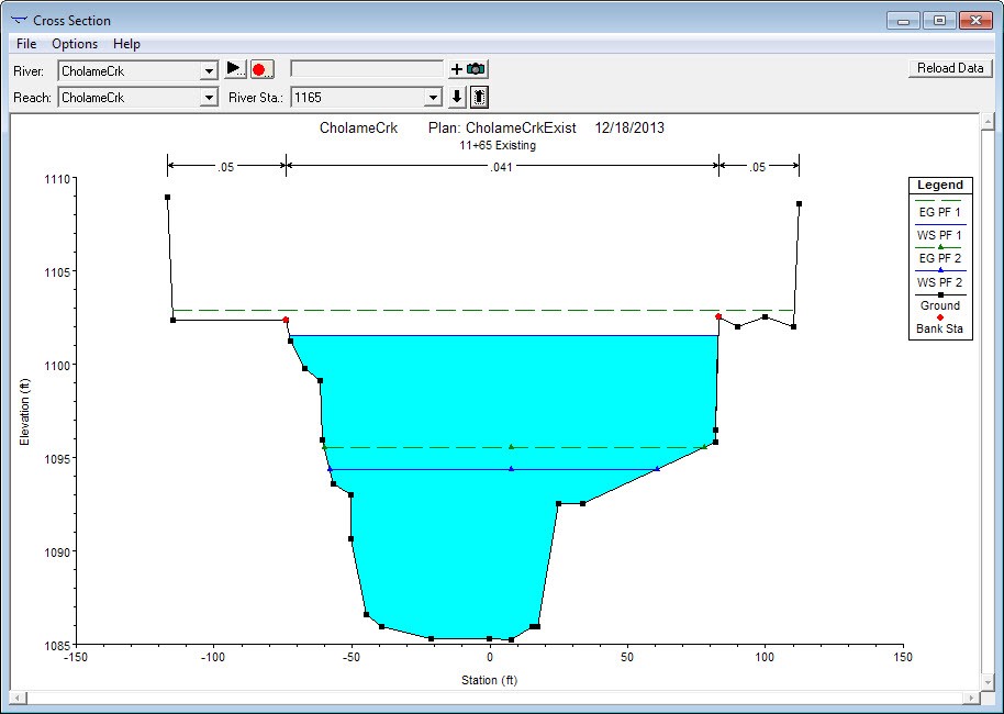
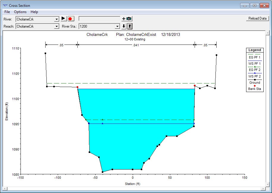
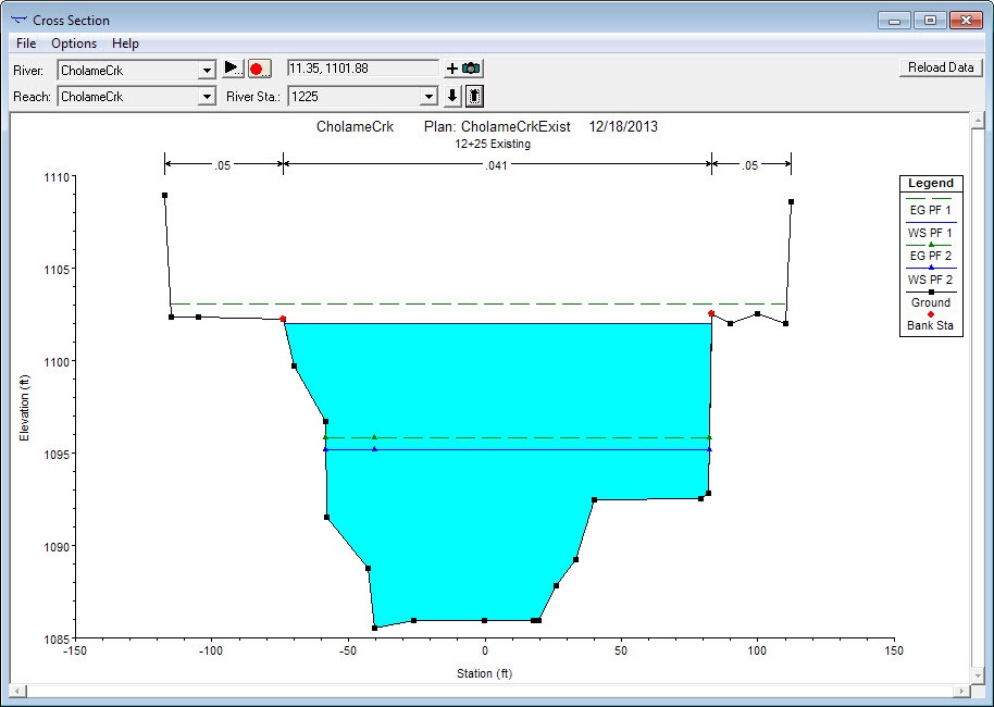
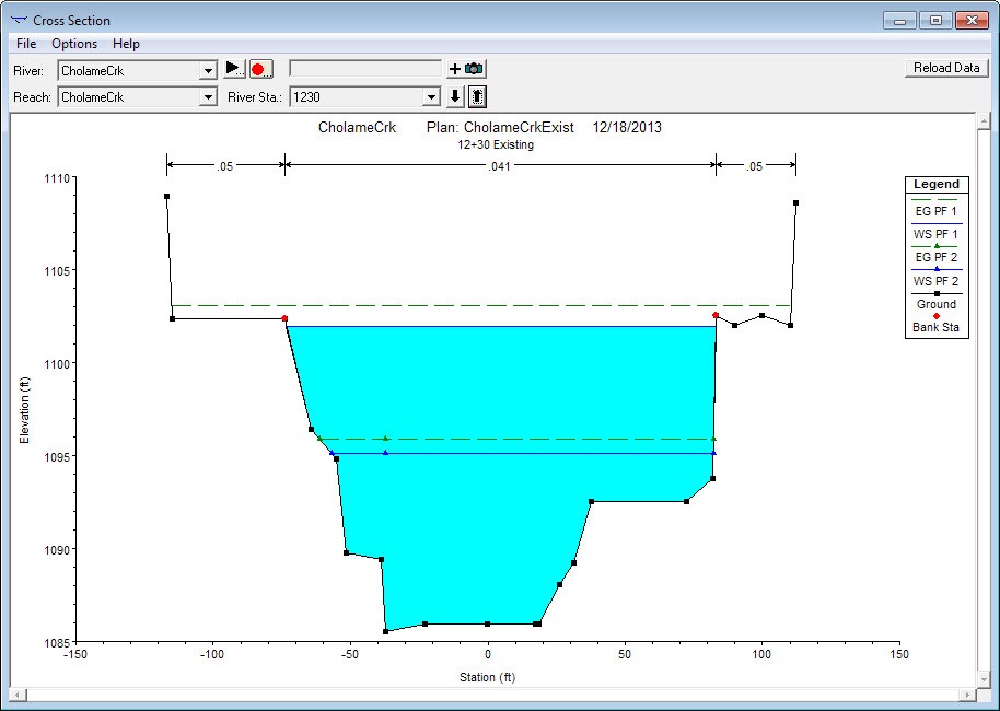
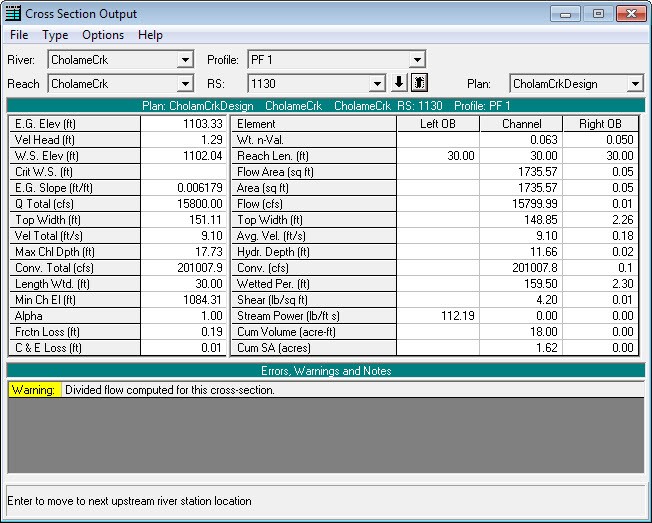
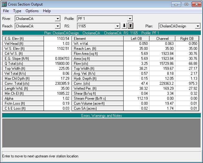
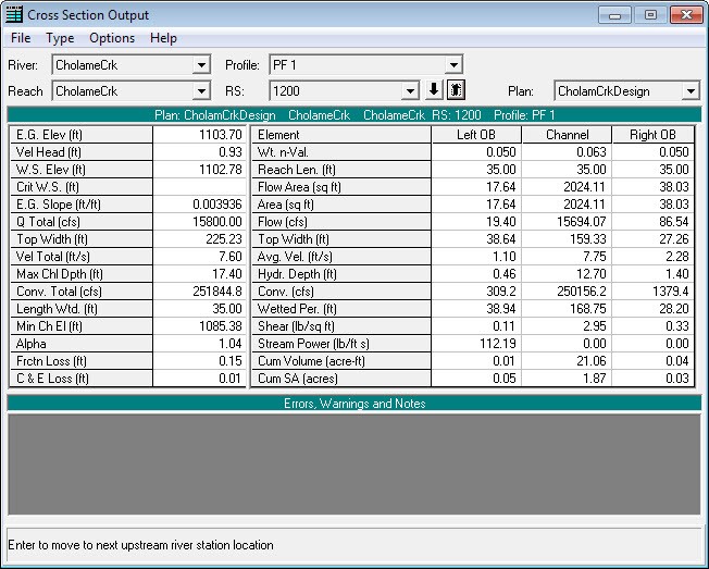
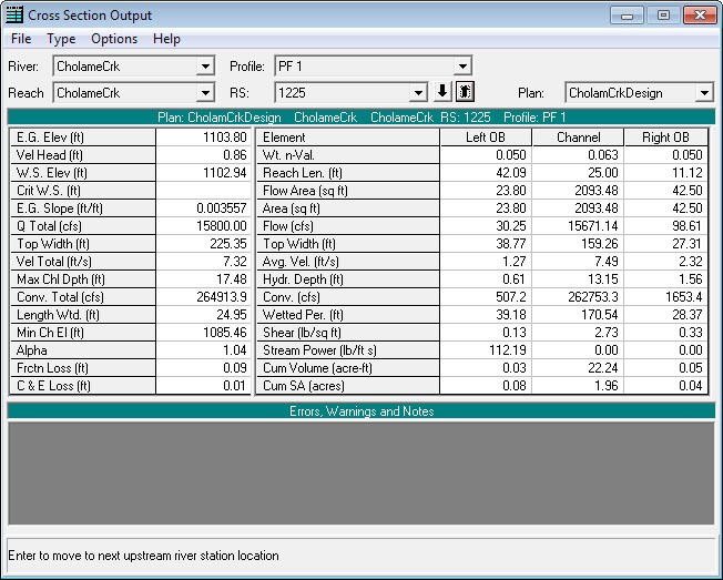
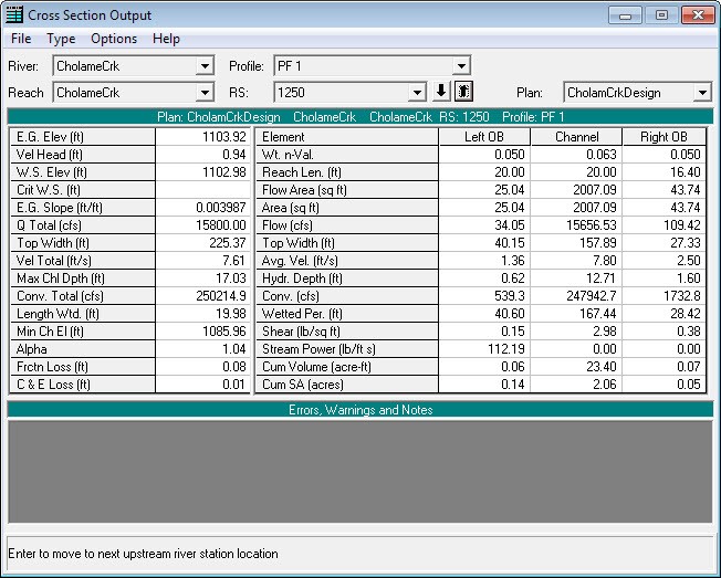
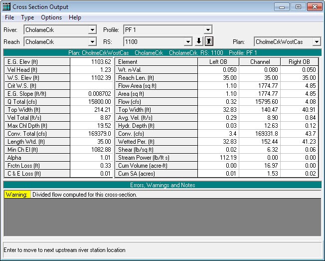
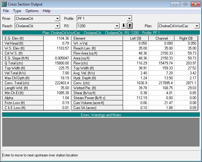
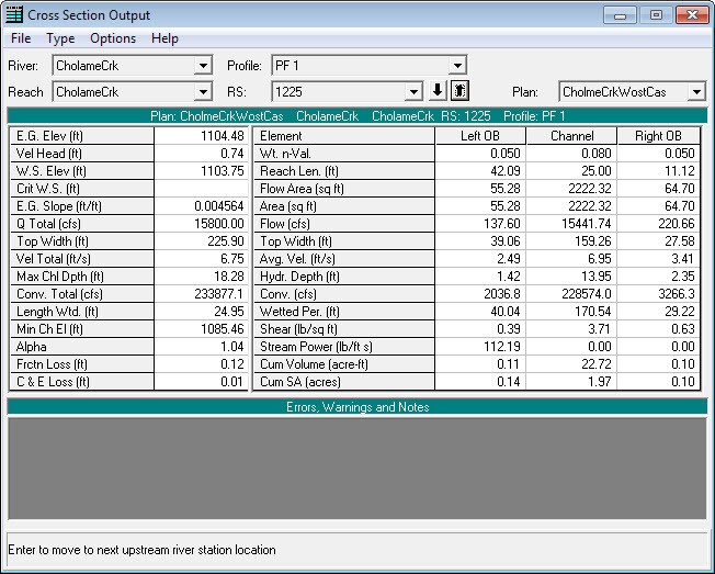
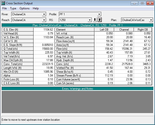
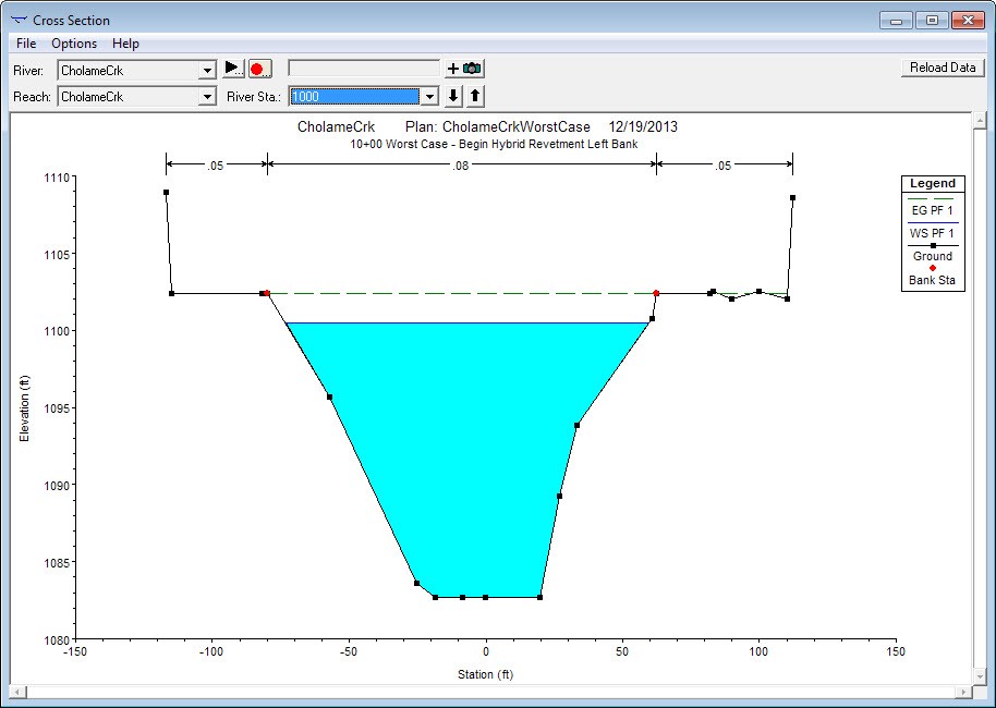
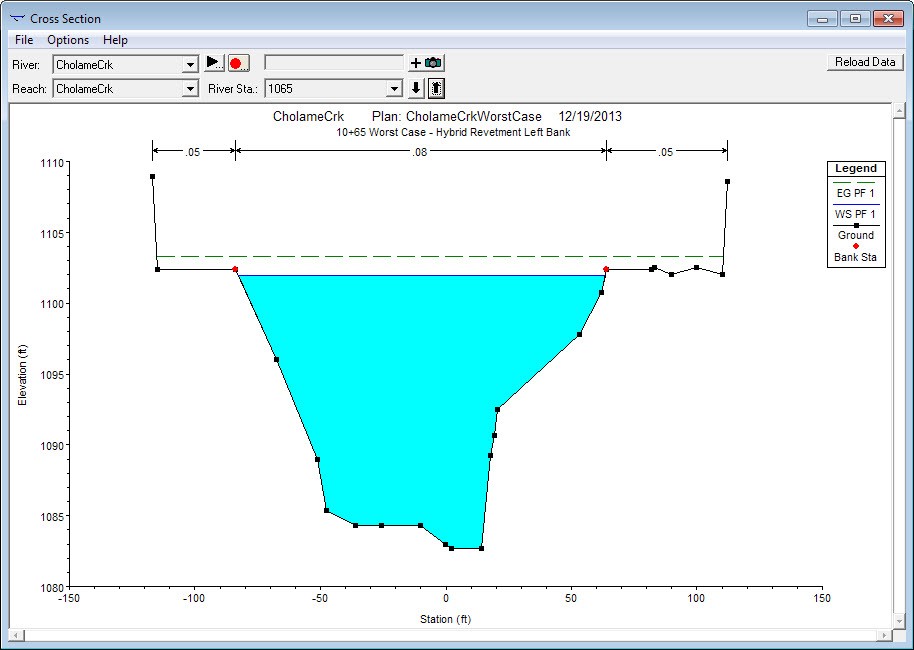
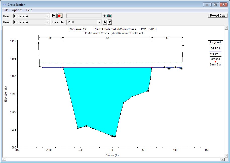
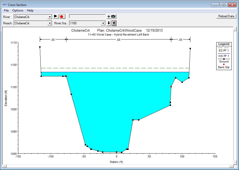
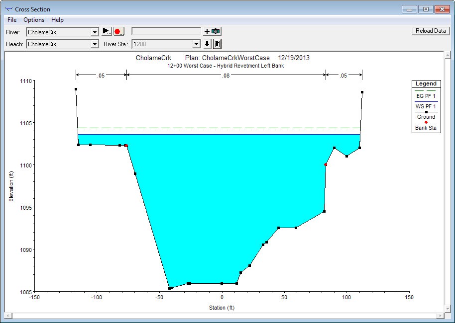
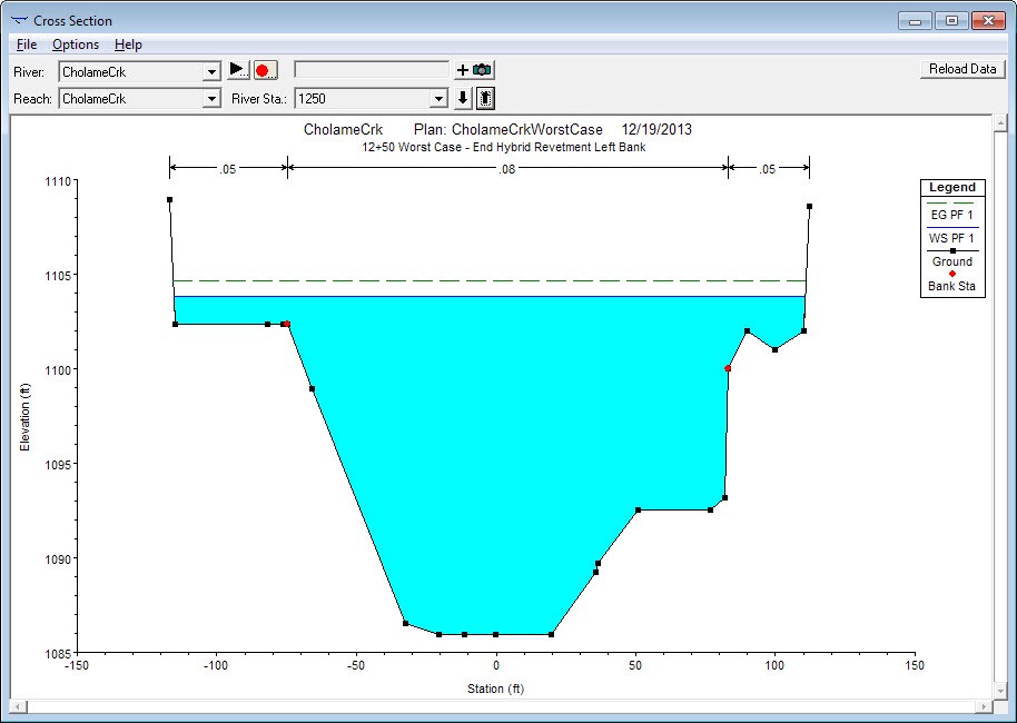
NOTE: In this Appendix, the HEC-RAS modeling output/results are only displayed for the hybrid revetment limits (STA 10+00 to STA 12+50) for each condition.

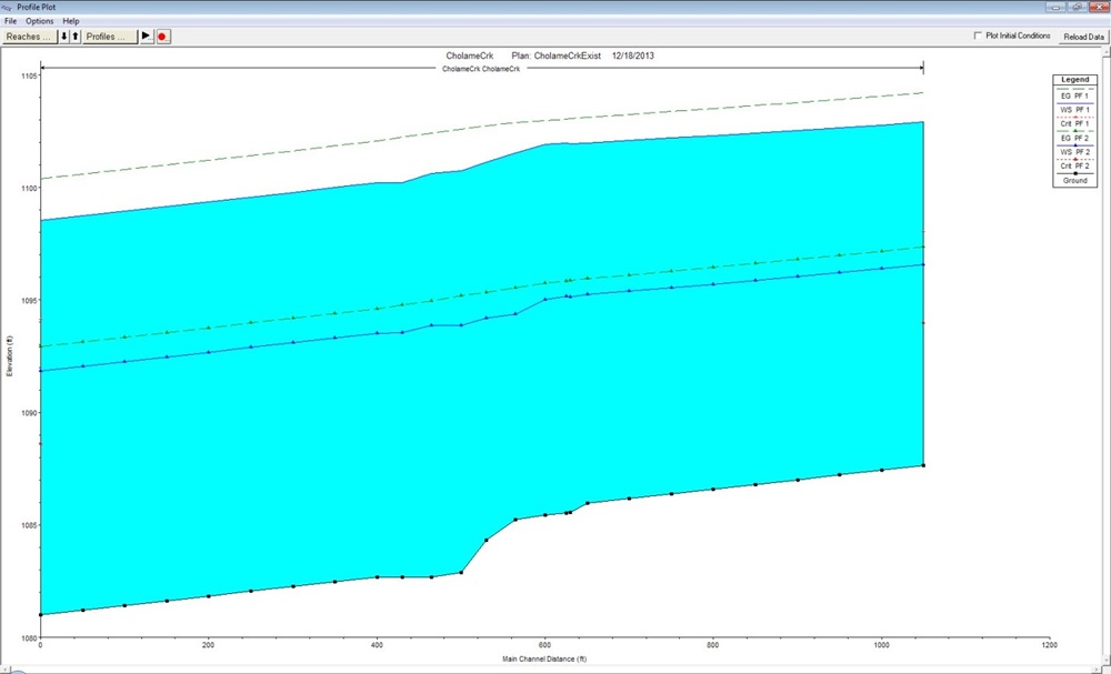
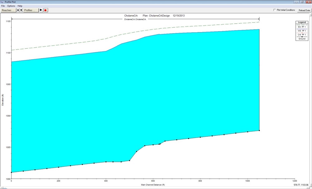
Pre-Construction Model

Post-Construction Model

Worst Case Scenario Model

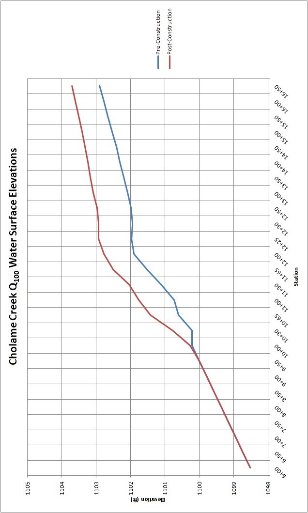
Sample Hydraulic Model Comparisons: Pre-Construction vs. Post-Construction

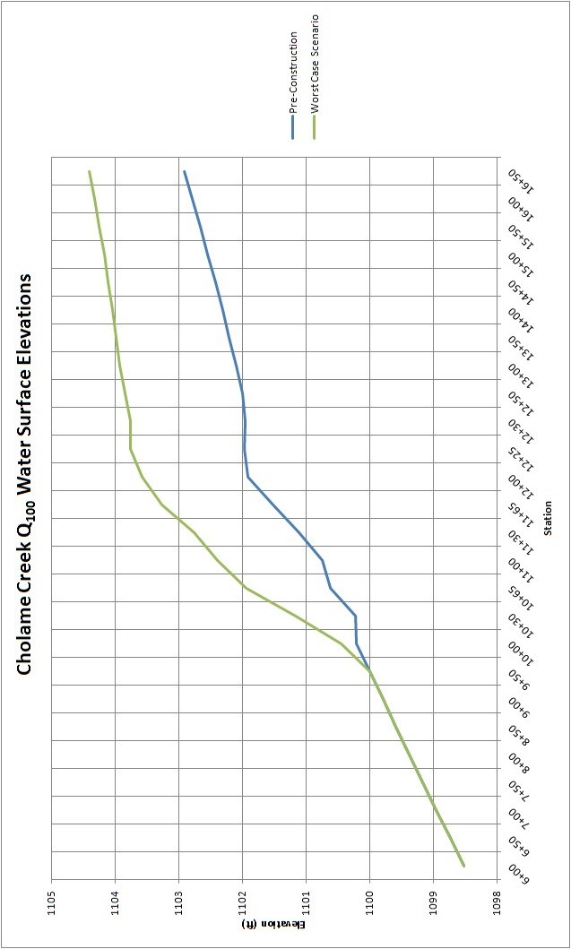
Sample Hydraulic Model Comparisons: Pre-Construction vs. Worse Case Scenario

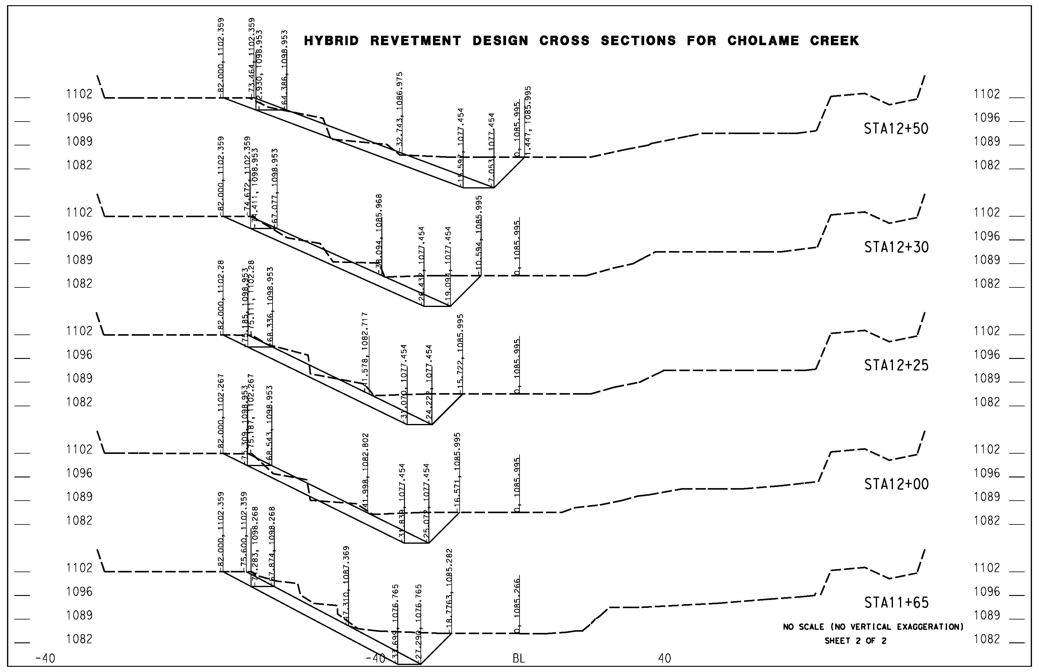
Appendix C - Sample Hybrid Revetment Plan Sheets and Design Cross Sections

Appendix D - Gravel Filter Nonstandard Special Provision

General

The gravel filter is associated with streambank rock slope protection (RSP) revetments and used as a buffer between native base soil and RSP to reduce base soil migration and promote free passage of subsurface drainage.

Gravel filter includes its placement on streambank subgrade as shown.

Materials

The gravel filter will consist of hard, durable, clean and washed, gravel, cobble, crushed stone, crushed rock, or any combination of these free from organic material, clay balls, or other deleterious substances.

The aggregate used in the gravel filter must have a durability index not less than 40 and must contain at least 90 percent crushed particles when tested under California Test 205.

The percentage composition by weight of gravel filter in place must comply with the grading requirements shown in the following table:

Gravel Filter Grading Requirements

Construction

Deliver uniform mixture of gravel filter to the site. Spread uniform mixture in layers and shape to thickness and limits shown using suitable equipment.

Local surface irregularities of the gravel filter aggregate must not vary from the planned slope by more than 2 inches as measured at right angles to the slope.

Payment

The quantity of gravel filter is based on the dimensions shown.