
Appendix D – San Diego Region Coastal Sea Level Rise Analysis
Executive Summary
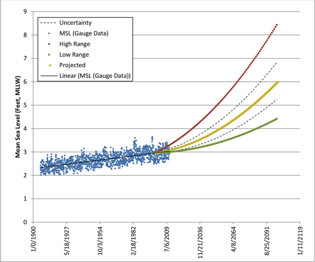
Sea level rise (SLR) has occurred on a global and local scale over the last century, and projections suggest that the rate might accelerate into future planning horizons (e.g., 2050 and 2100), as shown in Figure ES-1. Recently, projects being planned within the coastal zone have been required by regulatory, resource, and funding agencies to incorporate SLR considerations into project planning and design. Contingent on the project, incorporation of these SLR projections into project design can have significant impacts on the project relative to cost, the environment, wetlands encroachment, views, existing structures, right of way, and flood control; all of which will be fully evaluated in the identification of the Least Environmentally Damaging Practicable Alternative (LEDPA) during the environmental review and permitting phase of the project.
This report summarizes and compiles relevant state, federal, and local guidance for sea-level rise and provides recommendations of future ocean water levels for consideration by Project Development Teams (PDTs) in the design of the proposed transportation improvements associated with the North Coast Corridor (NCC) Program. This report was also prepared in accordance with SANDAG's Climate Action Strategy and addresses the NCC Program area of coastal San Diego County.
The NCC Program includes improvements to Interstate 5 from Oceanside to the University Town Center area, and on the LOSSAN railroad from Oceanside to Sorrento Valley, but does not include improvements to Highway 101. Highway 101 is the responsibility of the local agencies that it passes through. The proposed approach for Project Development Teams during the design of future improvements will consider the full range of SLR projections in the alternatives analysis phase over the design life of an individual project. Based on current scientific developments, regulations, and the results of these site-specific analyses, the preliminary design will either:
- accommodate SLR projections specified in local, state, and federal guidance documents in combination with flood flows;
- include adaptation strategies so that the structures can be raised in the future should the projections be realized; or
- consist of a risk assessment that may conclude the benefits of developing a design that fully accommodates SLR projects may be outweighed by the environmental and economic impacts of constructing such a project design, leading to a less conservative design and episodic operational constraints.
In March 2013, the State of California, via the California Climate Action Team and Ocean Protection Council, established the latest SLR guidance, which was based on the latest and most relevant scientific study presented in the 2012 National Research Council study (NRC 2012). The latest state guidance is to consider a range in SLR of 0.13 feet to 0.98 feet between 2000 (Base Year) and 2030, 0.39 feet to 2.00 feet between 2000 and 2050, and 1.38 feet to 5.48 feet between 2000 and 2100. The high end of the range is based on high fossil fuel usage, and the low end of the range is a change in lifestyle resulting in a lower mean sea level rise scenario. The guidance also recommends a site-specific risk analysis to inform the design and to determine the appropriate SLR projection for design. This risk tolerance approach is the most likely outcome for any NCC rail/highway bridge that can't accommodate the upper projection of SLR.
The NCC Program is a 40-year program of regional transportation improvement consisting of a series of individual projects planned to be implemented over four decades: 2010-2020, 2021-2030, 2131-2040, and 2041-2050. Bridges currently permitted met the requirements at the time they were permitted so any changes needed to address SLR for those bridges will be made in the future. Phase 1 bridges (implementation in the 2010-2020 decade) are being designed in consideration of current SLR science and guidance, with varying approaches consisting of
- complete consideration of SLR;
- partial consideration of SLR (if constrained) with future adaptation; or
- inability to accommodate SLR but with episodic, low-frequency operational constraints such as bridge closures when freeboards are exceeded. The estimated time for such closures is on the order of several hours rather than days. Bridges to be built in subsequent phases will be reassessed in the future and such assessment will be done in the context of SLR science and guidance available at that time. This document can be updated for each implementation phase to help maintain a consistent approach to addressing SLR for all NCC program components.
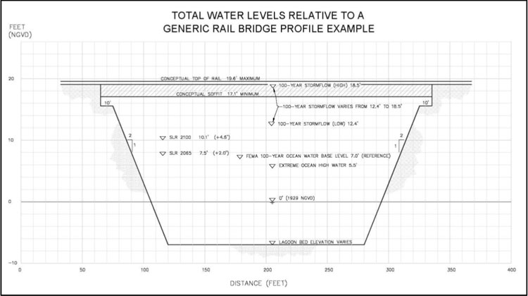
Guidance for design water levels for the NCC Program was provided across this range of future mean sea levels in consideration of high ocean water levels both with and without fluvial floods (50-year and 100-year). High future water levels that combine the extreme flood event with SLR of 1.5 feet, 3.0 feet, 4.6 feet, and 5.5 feet are compared to existing and proposed bridge elevations (I-5 and railroad) to assist PDTs in bridge design. For Highway 101 bridges, due to their proximity to the coastline, design water levels need to consider both fluvial floods under future mean sea levels and extreme wave crest elevations under future mean sea levels with the higher design water level used for bridge design. The report also discusses the potential impacts of tsunamis on the study area and recommends that the proposed improvements be designed to accommodate various influences of these phenomena. Such measures typically include using pile-supported structures, protecting embankments from scour, and securing precast elements from the uplift. Load combinations for tsunamis can consist of water levels due to tsunamis during ocean mean high water conditions, without a fluvial flood event. Figure ES-2 shows an example of the components of high water levels that affect bridge infrastructure design.
1.0 Introduction
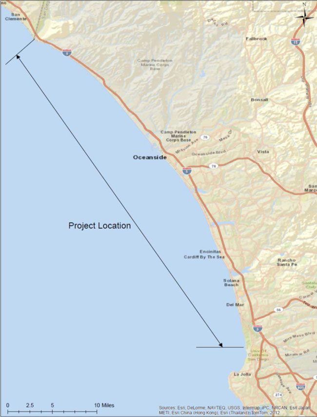
This document presents the processes to determine sea levels for the San Diego coastal region to be utilized for the design of transportation infrastructure associated with the proposed I-5 North Coast Corridor (NCC) Program including rail, roadway, and bridge improvements. The study area encompasses coastal areas from north San Diego County to just south of the I-5/I-805 merge, as shown in Figure 1-1.
This study was prepared in accordance with the San Diego Association of Governments (SANDAG) Climate Action Strategy (CAS) (SANDAG 2010a) that recommends consideration of climate change in the design of transportation infrastructure.
Specifically, the study is consistent with Goal 4 (Project Transportation Infrastructure from Climate Change Impacts), Objective 4b of the CAS, as listed below:
- Objective 4b: Protect Transportation Infrastructure from Sea Level Rise (SLR) and Higher Storm Surges. This objective includes the following policy measures:
- Develop a climate vulnerability plan that will identify areas in the San Diego region at risk of damage from SLR and storm surges;
- Modify standards for the design, location, and construction of infrastructure to account for areas potentially subject to storm surge, SLR, and more frequent flooding events;
- Reduce building in floodplains and areas subject to storm surge or SLR, or adequately protect structures in floodplains;
- Engage a multi-disciplinary team of climate change and coastal experts along with hydraulics and bridge design specialists during the scoping process of coastal bridge projects to consider localized effects;
- Identify adaptive management and monitoring to incorporate into regional transportation planning (SANDAG); and
- Address adaptation issues in the design and location of new projects and when improvements are made to existing infrastructure.
The NCC Program's goal is to meet a mobility vision defined in the 2050 Regional Transportation Plan that would serve to improve and maintain public transportation facilities of regional, state, and national significance. The NCC Program highway and rail improvements are described in detail in the public documents prepared for SANDAG and California Department of Transportation (Caltrans) as listed below:
- San Diego – Los Angeles to San Diego (LOSSAN) Corridor Project Prioritization Analysis (SANDAG 2009);
- SANDAG 2050 Regional Transportation Plan (SANDAG 2011); and
- North Coast Corridor Public Works Plan/Transportation Resource Enhancement Program (PWP/TREP) (SANDAG 2013).
The NCC Program improvements are being administered by SANDAG and Caltrans. The capital improvements in the LOSSAN Rail Corridor are being funded by the Federal Rail Authority (FRA), Federal Transit Authority (FTA), State of California, Amtrak, and local TransNet Program. Highway and freeway projects are being funded by the Federal Highway Administration (FHWA), Caltrans, State of California, and local TransNet Program. This study focuses on both roadway and railroad improvements along Interstate 5 and the LOSSAN rail corridor. Highway 101 is not included in the NCC Program but is included in this report for completeness.
2.0 Climate Change Science and Sea Level Rise Overview
The anticipated changes in climate and sea levels are a result of the build-up of "greenhouse" gases in the atmosphere over time due to emissions from the burning of fossil fuels for energy production and from natural sources. Greenhouse gases trap longwave thermal radiation within the Earth's atmosphere and warm the atmosphere and globe, which results in climate change and SLR. A schematic illustrating incoming shortwave radiation from the sun and outgoing, long-wave thermal radiation being partially trapped by the presence of greenhouse gases is shown in Figure 2-1.
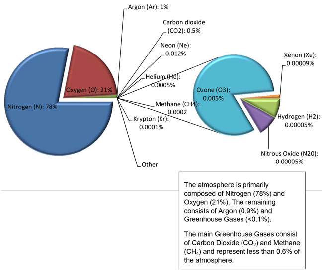
Atmospheric gas constituents in the atmosphere and their relative percentage of greenhouse gases are shown in Figure 2-2. Although greenhouse gases comprise less than a tenth of a percent of the atmosphere, the thermal effect of these gases is disproportionate to their relative percentages. Therefore, the warming of the atmosphere relative to the composition of these gases is a non-linear process. Carbon dioxide is the chief constituent of greenhouse gases.

2.1 Sea Level Rise Projections
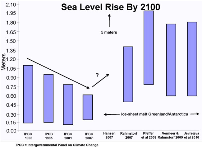
Global (i.e., eustatic) SLR refers to increases in the volume of water in the ocean principally related to thermal expansion and glacial ice sheet melt. There is a wide range of opinions and projections about global SLR rates due to the non-linear relationship between carbon dioxide build-up, thermal effects on the atmosphere, and climate change. An example of the disparity between the various SLR projections for the year 2100 is shown in Figure 2-3. Certain outliers (e.g., Hanson 2007) include parameters associated with glacial processes that result in much higher numbers (up to 5 meters). Although there is no probability assigned to SLR predictions at this time, some projections are being more widely adopted by agencies than others. Global SLR projections and agency guidance are discussed in detail in Section 3.0 of this study. A recently released study by the National Research Council (NRC) is presented that indicates the degree of uncertainty in the predictions, as discussed subsequently in this study.
In the Study area, the rate of global SLR is of less practical importance than the rate of SLR relative to the land. This concept is commonly referred to as relative SLR. The rate of relative SLR can be affected by:
- local ocean conditions (e.g., some parts of the ocean may be warming and, therefore, exhibiting rising water levels more rapidly than others);
- regional decadal oscillation patterns;
- land uplift or subsidence; and
- rates of sedimentation or erosion of an area.
This Study focuses on relative SLR in the local area as dictated by local conditions, referred to as local SLR. Local SLR is discussed in more detail in Section 5.2 of this study.
2.2 Project-Level Sea Level Rise Considerations
Consideration of SLR may be required through various project phases, including alternatives analysis, preliminary design, permitting, and final design. Recommendations for identifying and addressing SLR issues for the project include: 1) identifying whether the project could potentially be affected by future higher sea levels within its design life, and then 2) identifying all responsible agencies that might participate and their respective role(s).
Planners, engineers, and scientists have had a broad array of global SLR projections since the 1980s; however, specific agency guidance on how to incorporate SLR considerations into projects has only become available recently. The combination of varying SLR projections and multiple sets of agency guidance can complicate the design of coastal projects. Since multiple regulatory agencies need to be consulted to obtain project approvals, a comprehensive SLR guidance approach is necessary.
Regulatory and funding agency guidance were analyzed to determine the approach for the project. Basic project assumptions are as follows:
- Project start year of 2013 or later;
- Project design life is 100 years for the LOSSAN rail bridges and 75 years for the Interstate 5 Freeway (Highway 101 is not included in the NCC Program); and
- Principal funding agencies are SANDAG, Caltrans, FHWA, FRA, and FTA.
The relevant sea level guidance is organized in Table 2-1 by the various sponsoring agencies/organizations.
Table 2-1. Relevant Agency Sea Level Rise Guidance
| Agency/Organization | Sea level Rise Guidance | Applicable |
|---|---|---|
| SANDAG | Climate Action Strategy (2010a) | Yes |
| San Diego Region Coastal Sea Level Rise Analysis | Yes | |
| San Diego Bay bordering Cities, County, and Port | Sea Level Adaptation Strategy for San Diego Bay | Yes |
| Public Utilities Commission | None | — |
| Amtrak | None | — |
| CO-CAT | CO-CAT Guidance, 2013 | Yes |
| U.S. DOT | LaHood, 2011 | Yes |
| FRA | None | — |
| FHWA | HEC-25 | No |
| FEMA | FEMA 1991, 2004, 2005, 2010, 2011a | No |
| USACE | USACE 2009a, 2009b, 2011 | Yes |
These agencies/organizations have different types of involvement, including funding, administration and/or oversight, planning, regulatory review and approval, design, construction, monitoring, emergency preparedness, or multiple levels of involvement. Depending on the agencies/organizations involved in the specific projects that are a part of the NCC Program, the PDTs may need to consider other relevant guidance in addition to the guidance from this study.
3.0 Summary of Relevant Public Sea Level Rise Guidance
A technical review of available public guidance on SLR was conducted to provide applicable project planning and design information. Guidance is summarized in this section by the publication's origin (i.e., international/federal/state/local entities, and the scientific community) and date of release (earliest to most recent). Of note is that all guidance discussed in this section is in terms of global SLR rather than local SLR. Local SLR is specifically discussed in Section 5.2.
3.1 Internationally Recognized, Peer-Reviewed Literature
3.1.1 Intergovernmental Panel on Climate Change Projections
This section summarizes the two most recent reports released by the Intergovernmental Panel on Climate Change (IPCC). These reports provide SLR projections that were later incorporated into federal and state guidance documents.
3.1.1.1 Third Assessment Report (IPCC 2001)
The Third Assessment Report (TAR) of the IPCC is a detailed synthesis of the available peer-reviewed science. It is similar to the subsequent Fourth Assessment Report in being consensus-driven and potential contributions to SLR are not included unless there is broad agreement that they are quantitatively understood.
The TAR projects a SLR of 4 to 35 inches (10 to 89 centimeters [cm]) between 1990 and 2100. As with the Fourth Assessment Report, the largest contribution to the uncertainty is associated with modeling uncertainties and, in particular, with the potential for dynamic ice sheet instability. The West Antarctic Ice Sheet is particularly called out in regard to uncertainty.
3.1.1.2 Fourth Assessment Report (IPCC 2007)
The Fourth Assessment Report (4AR) of the IPCC contains a detailed synthesis of the available peer-reviewed science of climate change and sea-level modeling and has received contributions and comments from a vast array of respected researchers in the field. This document is discussed at some length herein because it is the baseline for most other assessments, even those critical of its results.
The 4AR gives a widely quoted projection of 7 to 23 inches (18 to 59 cm) for SLR in the 21st Century. These are considered to be 5 to 95 percent confidence ranges. The 4AR includes a second set of projections – from 7 to 30 inches (18 to 76 cm), which includes a scaled-up ice discharge term. The projections cover the period from 1990 to the midpoint of 2090-2099. The 4AR does not provide SLR values at intermediate periods (e.g., to 2050).
The models described in the 4AR give reasonable hindcasts of observed SLR between 1993 and 2003, although they under-predict observed SLR between 1961 and 2003.
The uncertainty in the quoted projections derives from two main sources:
- Different greenhouse gas emission scenarios. The IPCC defines six future scenarios of the world population and economy that predict different levels of greenhouse gas emissions. The 4AR stresses that no scenario can be considered more likely than others.
- The second, and larger, uncertainty is associated with limitations to current scientific knowledge. The range of SLR projections for a given scenario is based on the range of results from 17 independently developed and peer-reviewed general circulation models.
Compared to the TAR, the projections in 4AR are slightly smaller and significantly narrower. The "headline value" from the TAR was 4 to 35 inches (10 to 89 cm) between 1990 and 2100. The reasons for the differences are as follows:
- The projections in the 4AR are to the midpoint of the period 2090 to 2099, while those in the TAR are to 2100;
- The TAR included some small additional contributions (e.g., 0.2 inch [0.5 cm]) based on the additional rise in the 21st Century due to permafrost, which is not included in the 4AR; and
- The 4AR modeling uncertainties have been decreased with improved information and modeling capabilities. The TAR uses simple climate models to estimate SLR; these are less detailed than the atmosphere-ocean general circulation models used in the 4AR.
Mechanisms that may lead to SLR are not included in the 4AR projections unless there is a broad scientific consensus that they are well and quantitatively understood. That is, the 4AR projections are conservative in a scientific sense, but not in an engineering or planning sense. The 4AR freely admits that it may under-predict as well as over-predict future SLR. In particular, the projections do not include potentially large and nonlinear effects such as a potential nonlinear instability and accelerated loss of the Antarctic and Greenland Ice Sheets – because there are no broadly accepted models of these processes. It is not even known whether ice sheet discharge will increase or decrease SLR in the short-term. The projections do include the best current understanding of polar ice dynamics.
Critics of the IPCC have generally focused on this scientific conservatism. In particular, many planners have expressed concern that the projections are not sufficiently conservative in an engineering sense, and that the upper limits of the IPCC projections do not represent a worst-case scenario. However, the scientific community generally has not attempted further synthesis of the huge range of available models and potential contributions to future SLR; as a result, few hard numerical predictions of total SLR have been published in the peer-reviewed literature since dissemination of the 4AR.
3.2 Federal Guidance
Several federal SLR guidance documents have been prepared and are summarized below. The latest U.S. Army Corps of Engineers (USACE) guidance (2011) and NRC (2012) study are the most applicable to the project. However, it should be noted that the USACE guidance only applies to USACE led, civil works projects. State SLR guidance is currently being updated and it is our understanding that the NRC (2012) study projection will be the basis of this revision.
3.2.1 U.S. Army Corps of Engineers, Engineering Circular No. 1165-2-211 (2009a)
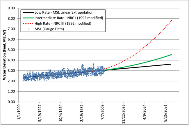
Engineering Circular (EC) No. 1165-2-211 issued by the USACE recommends evaluation of three scenarios in planning civil works projects potentially affected by SLR:
- Low Rate – future rates of sea-level change is based on historical trends in local mean sea level, which are best determined by tide gauge records greater than 40 years in duration;
- Intermediate Rate – modified NRC Curve I (1.7 feet [0.5 meters] in 2100), considers both the most recent IPCC projections and modified NRC projections; and adds those to the local rate of vertical land movement; and
- High Rate – modified NRC Curve III (5.0 feet [1.5 meters] in 2100), considers both the most recent IPCC projections and modified NRC projections and adds those to the local rate of vertical land movement. This high rate exceeds the upper bounds of IPCC 2001 and 2007 estimates and accommodates the potential rapid loss of ice from Antarctica and Greenland.
This is a straightforward method of projecting SLR. The NRC curves were originally estimated in 1987 and estimates can be compared to actual sea levels measured since that time.
3.2.2 U.S. Army Corps of Engineers, National Vertical Datum (2009b)
The USACE established its policy for referencing project elevation grades to nationwide vertical datums established and maintained by the U.S. Department of Commerce (USACE 2009a). The current reference datum is the North American Vertical Datum of 1988 (NAVD88) and the water level reference is the National Tidal Datum Epoch of 1983 – 2001. The Engineer Manual (USACE 2010) provides detailed guidance for referencing datums on civil works projects.
3.2.3 Federal Emergency Management Agency (2010)
The Federal Emergency Management Agency (FEMA), a part of the U.S. Department of Homeland Security, administers the National Flood Insurance Program (NFIP) and the National Infrastructure Protection Plan (NIPP).
The NFIP offers federal flood insurance in participating communities that meet minimum floodplain management requirements in order to mitigate flood losses. In participating communities, FEMA prepares flood risk maps delineating flood risk zones that coincide with insurance premiums. Currently, FEMA does not specifically require addressing SLR as part of the NFIP and flood insurance studies. However, climate-change-related SLR is indirectly incorporated into the NFIP through various requirements and incentives (FEMA 1991, 2000, 2004, 2005, 2010, 2011a, 2011b). FEMA is researching climate change and impacts to the NFIP that includes a National Climate Change Study, which is anticipated for completion in 2012 and may revise FEMA's policy on SLR.
The NIPP was designed to ensure the resiliency of critical infrastructure and key resources of the United States from catastrophic loss from terrorist attacks and natural, manmade, or technological hazards. The NIPP provided guidance for many specific risks but does not address threats from SLR or climate change (NIPP 2009).
FEMA also addresses impacts from SLR based on mapping of high-risk areas, with more emphasis on flood risk. FEMA maps only contain current conditions, not future or projected conditions. Hence, FEMA periodically updates maps of high-risk areas for informational purposes. In 2010, FEMA conducted a proof-of-concept study to generate a SLR advisory layer as a follow-on product to their normal flood risk maps and flood insurance studies. Conceptually, the SLR map would be non-regulatory and would be intended to help states and communities identify and adapt to potential increases in the risk of flooding hazards.
3.2.4 U.S. Department of Transportation (2011)
The U.S. Department of Transportation (USDOT) climate change policy is to incorporate climate change adaptation strategies into its transportation missions, programs, and operations (LaHood 2011). The Transportation and Climate Change Clearinghouse within the USDOT coordinate the research on climate change and impacts on transportation systems. Enforcement of the USDOT climate change policy is left to each modal administration within the USDOT.
The FHWA is a division within the USDOT. The FHWA provides guidance for the analysis, planning, design, and operation of highways. Currently, the FHWA does not require consideration for SLR in the design of bridges. Guidance for bridge design is published in hydraulic engineering circulars (HEC) and SLR is discussed in HEC-25 (Douglass and Krolak 2008). The target audiences for HEC-25 are engineers, designers, inspectors, and planners who are expected to fulfill professional obligations to seek out and utilize relevant project guidance.
3.2.5 Federal Rail Authority
The Federal Rail Authority does not possess specific guidance on SLR. Research into this potential guidance did not generate applicable information.
3.2.6 U.S. Army Corps of Engineers, Engineering Circular No. 1165-2-212 (2011)
The EC No. 1165-2-212 provides guidance on the consideration of the direct and indirect physical effects of SLR across the project life cycle for civil works projects. Under this EC guidance, the following should be considered:
- The degree to which systems are sensitive and adaptable to climate change and other global changes, including a) natural and managed ecosystems; and b) human and engineered systems. The following documents were recommended for consideration in addressing these topics:
- a) The Climate Change Science Program Synthesis and Assessment Product 4.1 "Coastal Sensitivity to Sea-Level Rise: A Focus on the Mid-Atlantic Region" – presents the most recent knowledge on regional implications of rising sea level and possible adaptive responses.
- b) The National Research Council's (NRC 1987) report "Responding to Changes in Sea Level: Engineering Implications" – outlines a multiple scenario approach to deal with uncertainties for which no reliable or credible probabilities can be obtained.
- Three SLR scenarios (low, intermediate, and high) over the project life cycle. These three scenarios are as follows:
- Low Rate – the historical rate of SLR extrapolated from tide gauge records over the project life;
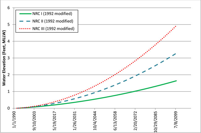
- Intermediate Rate – this is the modified NRC Curve I and Equations 1 and 2 (Figure 3-1) added to the local rate of vertical land movement.
E(t) = 0.0017t + bt2 (Equation 1)
E(t2) – E(t1) = 0.0017(t2-t1) + b(t22-t12) (Equation 2)
Where:
E(t) = the global SLR, in meters, as a function of t.
b = constant given for each of the three NRC (1987) curves.
t1 = time between the project's construction date and 1992.
t2 = t1 + number of years after construction.
These equations assume a global mean SLR estimate of 0.067 inches/year (1.7 millimeters/year), and that projects will be constructed at some date after 1992. - High Rate – this is the modified NRC Curve III and Equations 1 and 2 (Figure 3-1) added to the local rate of vertical land movement. Note that the high rate exceeds the upper bounds of IPCC estimates from both 2001 and 2007 to accommodate the potential rapid loss of ice from Antarctica and Greenland, but is within the range of peer-reviewed articles released since that time.
- Evaluate the sensitivity of alternative plans and designs to future mean SLR. There are many ways to address this comparison and selection step. Examples are as follows:
- Use a single SLR scenario and identify a preferred alternative under this scenario. This approach is best when conditions and plan performance are not very sensitive to the rate of SLR.
- Compare all alternatives against all SLR scenarios.
- Select a plan which provides a way forward to address uncertainty. This could be in the form of a sequence of decisions allowing for adaptation based on evidence.
3.2.7 National Research Council (2012)
The 2012 NRC report updates the 4AR with estimates of global and, specifically, U.S. West Coast (California, Oregon, and Washington) SLR projections. The study divided the U.S. West Coast into two zones (north and south of Cape Mendocino) due to their differing tectonic characteristics and consequent vertical land movement. The area north of Cape Mendocino (Cascadia region) is generally rising, while the area south of Cape Mendocino (San Andreas region) is generally sinking. The study made the following findings for the region south of Cape Mendocino, which includes this study area:
- Tide gages indicate variability in sea-level change along the coast, although most of the gages show that relative SLR has been rising over the past 6-10 decades;
- Vertical land motion (based on GPS measurements) suggests that the coast is sinking at an average rate of about 0.04 inches (1 mm) / year;
- Factors that affect local SLR for this region include: thermal (steric) variations; wind-driven differences in ocean heights; gravitational and deformational effects (SLR fingerprints) of melting of ice from Alaska, Greenland, and Antarctica; and vertical land motions along the coast; and
- Regional SLR projections are less certain than global ones because there are more components to consider.
The NRC study predicts a 0.9-foot increase in SLR by 2050 and a 2.7-foot increase by 2100 globally, as shown in Table 3-1 and Figure 3-2. Regionally, the study predicts the Southern California region will track closely with global SLR estimates. Projections were produced for the Los Angeles region, which was estimated at a 0.5-foot increase in SLR by 2050 and a 3.1-foot increase by 2100 (Table 3-2).
Table 3-1. NRC 2012 Global SLR Projections
| Year | Projection (ft) | Uncertainty (ft, +/-) | Low Range (ft) | High Range (ft) |
|---|---|---|---|---|
| 2030 | 0.4 | 0.1 | 0.3 | 0.8 |
| 2050 | 0.9 | 0.1 | 0.6 | 1.6 |
| 2100 | 2.7 | 0.3 | 1.7 | 4.6 |
Table 3-2. NRC 2012 Regional SLR Projections (Los Angeles)
| Year | Projection (ft) | Uncertainty (ft, +/-) | Low Range (ft) | High Range (ft) |
|---|---|---|---|---|
| 2030 | 0.5 | 0.2 | 0.2 | 1.0 |
| 2050 | 0.9 | 0.3 | 0.4 | 2.0 |
| 2100 | 3.1 | 0.8 | 1.5 | 5.5 |
The study provides both uncertainties as well as high and low ranges for each of the projections. The uncertainty and ranges are a function of the various global emission scenarios and ocean response mechanisms. The study suggests much higher confidence in the shorter time horizon years (i.e., 2030 and 2050) and a much lower confidence level in the 2100 projection.
3.3 State Guidance
Several SLR guidance documents have been prepared by the State of California. These documents are summarized in this section by the agency and in order of release date (earliest to most current). The most recent document was prepared by the Coastal and
Ocean Working Group of the California Climate Action Team (CO-CAT) with science support provided by the Ocean Protection Council's Science Advisory Team and the California Ocean Science Trust, and was issued in March 2013 and is currently considered the state SLR guidance. That document is presented below in this section.
3.3.1 California Coastal Commission (2001)
The California Coastal Commission's paper titled "Overview of Sea Level Rise and Some Implications for Coastal California" (CCC 2001) recognized that the continued rise in sea level will affect almost all coastal systems by increasing the inundation of low coastal areas and increasing the potential for storm damage, beach erosion, and beach retreat. Regarding implications, the report states that:
"In California, it is likely that a combination of hard engineering, soft engineering, accommodation/adaptation, and retreat responses will be considered to address sea-level rise. There are situations where each response may be appropriate and well suited. In all coastal projects, it is important to recognize and accept that there will be changes in sea level and other coastal processes over time."
3.3.2 Governor's Executive Order S-3-05 (2005)
The Governor's Executive Order (EO) S-3-05, issued on June 1, 2005, primarily addressed the establishment of greenhouse gas reductions; however, it did acknowledge the potential climate change-related impacts associated with rising sea levels. The EO specifically states that "…rising sea levels threaten California's 1,100 miles of valuable coastal real estate and natural habitats."
3.3.3 Governor's Executive Order S-13-08 (2008)
EO S-13-08 issued by Governor Arnold Schwarzenegger on November 14, 2008, recognizes the impact that SLR may have on coastal development in California. This order provides information from the longest continuous sea-level gauge at Fort Point, San Francisco which recorded a 7-inch rise in sea level in the 20th Century. Further, the IPCC (2007) predicted a global SLR between 7 and 23 inches in the 21st Century.
The EO directed the California Resources Agency to request that the National Academy of Sciences convene an independent panel to complete the first California SLR Assessment report. This report is the NRC 2012 report described above. The EO states that prior to the release of the final SLR Assessment Report, all state agencies planning construction projects in areas vulnerable to future SLR shall, for the purposes of planning, consider a range of SLR scenarios for the years 2050 and 2100 in order to assess project vulnerability and, to the extent feasible, reduce expected risks and increase resiliency to SLR.
SLR estimates should be used in conjunction with appropriate local information regarding local uplift and subsidence, and coastal erosion rates, predicted higher high water levels, storm surge, and storm wave data.
This EO specifies that a new study to be done by the NRC will set permanent guidance and supersede the interim guidance.
3.3.4 Climate Change Impacts Assessment (2008)
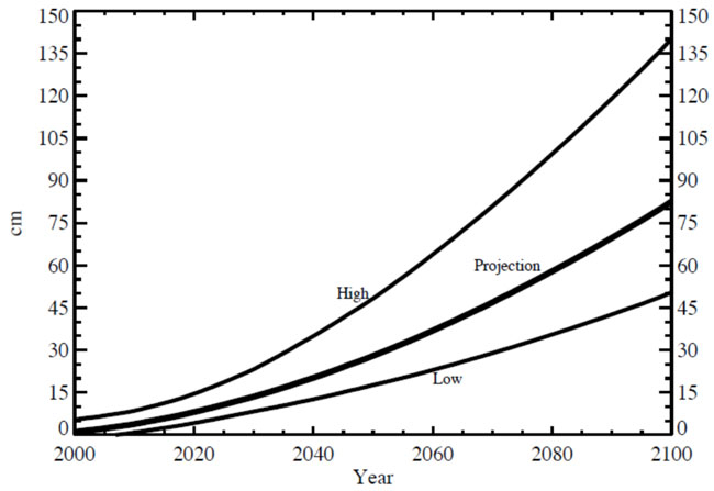
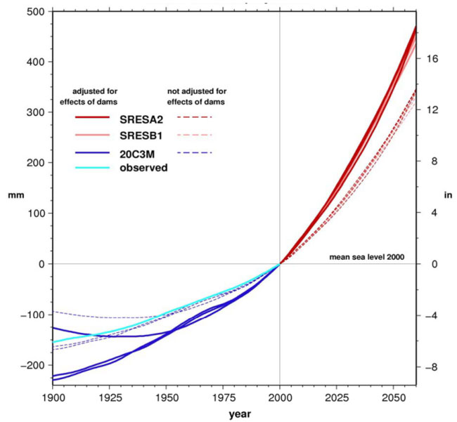
The biannual scientific reports overseen by CO-CAT serve as the primary basis for quantifying SLR projections in California as mandated by EO S-13-08. The first climate change impact assessment included estimates of SLR as published by the California Climate Change Center (CCCC) in 2006. The 2008 Climate Change Impacts Assessment (2008 Assessment) is the second of these biannual scientific reports. The 2008 Assessment is comprised of 40 studies and reports conducted by the CCCC for the California coast (CCCC 2009 & 2009a). The methodology for these SLR projections was based on the method of Rahmstorf (2007) applied to IPCC scenarios. For the 2008 Assessment, it was assumed that SLR along the California coastline was the same as global SLR and accounting for the global growth of dams and reservoirs that trap water was added. The 2008 Assessment SLR projections are shown in Figure 3-3 (CCCC 2009a). SLR projections above the 2000 water level for the year 2050 ranged from 12 to 18 inches (30 to 45 cm) and for the year 2100 ranged from 20 to 55 inches (50 to 140 cm).
3.3.5 California Climate Adaptation Strategy
The 2008 Assessment SLR projections were the basis for the reports titled The Impacts of Sea-level Rise on the California Coast (CCCC 2009b) and California Climate Adaptation Strategy by the California Natural Resources Agency (2009, 2010). The latter report was initiated by EO S-13-08 to develop California's first statewide climate change adaptation strategy to assess expected climate change impacts and recommend climate adaptation policies. This adaptation strategy is based on a projected sea-level rise of 55 inches (140 cm) by 2100 under the A2 IPCC climate change scenario. The strategy led to the adoption of a recent amendment to the California Environmental Quality Act (CEQA) Guideline, Section 15126.2, which requires lead agencies "to analyze how future climate change may affect development under the general plan."
Departments within the California Natural Resources Agency include the California Conservation Corps, Department of Boating and Waterways, Department of Conservation, Department of Fish and Game, Department of Parks and Recreation, Department of Resources, Recycling and Recovery, and Department of Water Resources.
3.3.6 California State Coastal Conservancy Memo (2009)
The California State Coastal Conservancy (CSCC) adopted a Climate Change Policy on June 4, 2009, which includes the following direction applicable to projects funded by the CSCC:
"Prior to the completion of the National Academy of Sciences report on SLR, consistent with Executive Order S-13-08, the Conservancy will consider the following SLR scenarios in assessing project vulnerability and, to the extent feasible, reducing expected risks and increasing resiliency to SLR:
- 16 inches (40 cm) by 2050; and55 inches (140 cm) by 2100.
3.3.7 Coastal and Ocean Working Group of the California Climate Action Team Interim Guidance (2010)
The State of California Sea-level Rise Interim Guidance Document (Interim Guidance) was released in October 2010 to provide guidance to state agencies for the incorporation of SLR projections into planning decisions prior to the release of the National Academy of Sciences (NAS) California SLR Assessment Report and is intended to enhance consistency among state agencies (CO-CAT 2010). The Interim Guidance was developed by the Sea Level Rise Task Force of the CO-CAT, with science support provided by the California Ocean Protection Council's Science Advisory Team and the California Ocean Science Trust. CO-CAT is comprised of senior staff from various California state agencies with ocean and coastal resource management responsibilities. The Sea Level Rise Task Force is comprised of staff from the following California agencies:
- The Business, Transportation and Housing Agency;
- California Coastal Commission;
- Department of Fish and Game;
- Department of Parks and Recreation;
- Department of Public Health;
- Department of Toxic Substances Control;
- Department of Transportation (Caltrans);
- Department of Water Resources;
- Environmental Protection Agency (CalEPA);
- Governor's Office of Planning and Research;
- Natural Resources Agency;
- Ocean Protection Council (OPC);
- San Francisco Bay Conservation and Development Commission;
- State Coastal Conservancy (SCC);
- State Lands Commission (SLC); and
- The State Water Resources Control Board.
The Interim Guidance includes policy recommendations agreed upon by the Sea Level Rise Task Force members. The recommended SLR projections are based on the Vermeer and Rahmstorf 2009 values, adjusted to the year 2000 baseline. The Vermeer and Rahmstorf 2009 SLR projections were based on a second-order, semi-empirical method correlating modeled global temperatures to SLR from 1990. The Vermeer and Rahmstorf 2009 SLR projections were reduced by 0.112 feet (0.034 meters) to adjust the 1990 baseline to a 2000 baseline (i.e., remove 10 years of SLR that has occurred from 1990 to 2000).
The Interim Guidance recommends that SLR projections, as summarized in Table 3-3, should be used as a starting place, and SLR value selection should be based on agency and context-specific considerations of risk tolerance and adaptive capacity. SLR projections are provided for the years 2030, 2050, 2070, and 2100. Projections for the years 2070 and 2100 include three ranges of values for low, medium, and high greenhouse gas emissions scenarios corresponding to the IPCC (2007) scenarios designated as B1, A2, and A1FI, respectively, and defined in subsequent section 3.5.2 of this report.
Table 3-3. Interim Guidance SLR Projections
| Year | Description | Average of Models in (cm) | Range of Models in (cm) |
|---|---|---|---|
| 2030 | 7 (18) | 5-8 (13-21) | |
| 2050 | 14 (36) | 10-17 (26-43) | |
| 2070 | Low | 23 (59) | 17-27 (43-70) |
| Medium | 24 (62) | 18-29 (46-74) | |
| High | 27 (69) | 20-32 (51-81) | |
| 2100 | Low | 40 (101) | 31-50 (78-128) |
| Medium | 47 (121) | 37-60 (95-152) | |
| High | 55 (140) | 43-69 (110-176) |
Additional recommendations regarding SLR projections include:
- Consider timeframes, adaptive capacity, and risk tolerance when selecting estimates of SLR;
- Coordinate with other state agencies when selecting values of SLR and, where appropriate and feasible, use the same projections of SLR;
- Future SLR projections should not be based on linear extrapolation of historical sea-level observations;
- Consider trends in relative local mean sea level;
- Consider storms and other extreme events (e.g., storm surge, El Niño, and wave setup); and
- Consider changing shorelines.
3.3.8 California Department of Transportation (2011)
In May 2011, Caltrans published its Guidance on Incorporating Sea-level Rise for use in the planning and development of project initiation documents (Caltrans 2011). Caltrans participated in the Sea Level Rise Task Force of the CO-CAT, which developed the Interim Guidance and 2013 Guidance documents. Hence, Caltrans guidance utilizes a portion of the SLR projections from the 2013 Guidance; specifically, the column labeled "Average of Models" in Table 3-3.
3.3.8.1 Sea Level Rise Impact Assessment
The guidance recommends analysis of potential SLR impacts and determination of whether SLR adaptation measures should be incorporated into the project. This determination is based on the level of risk and should be documented in a project initiation document. Each project should be initially screened to determine if there is a potential to be impacted by SLR, generally based on the following three questions:
- Is the project located on the coast or in an area vulnerable to SLR?
- Will the project be impacted by the projected SLR scenarios?
- What is the design life of the project?
If the project is located in the coastal zone and could potentially be impacted by SLR then the Project Initiation Document (PID) must contain a discussion on SLR.
3.3.8.2 Selecting Sea Level Rise Values for Caltrans Project Design
If it is determined that SLR could impact the project, then an analysis should be performed weighing the level of risk and potential for SLR-related consequences. If it is determined that SLR should be incorporated into a project, SLR projections are to be based on the 2013 Guidance (Table 3-3). SLR considerations should incorporate the following:
- Adjustments may be required for local subsidence or uplift;
- Adjustments may be required from the 2000 baseline;
- For a design life up to 2050, use value from "Average of Models";
- For projects with a design life beyond 2070, use the range of the three, "Average of Models";
- For design life years not provided in the Interim Guidance, linearly interpolate values in the table;
- SLR impacts are not needed for a project design life earlier than 2030; and
- SLR values for projects which include a new bridge or other major structures should choose a future date commensurate with the life of the structure (e.g., 75 years or more).
Currently, the Caltrans guidance only addresses changes to sea level. Due to the level of uncertainty, guidance has not yet been established for other climate change impacts such as changes to temperatures, storm intensity, storm surge, wave heights, precipitation patterns, and precipitation intensities. As more information becomes available on climate change, additional guidance is expected.
Once a determination has been made that SLR should be incorporated into the project, the PDT will need to conduct studies to estimate the degree of potential impact and assess alternatives for preventing, mitigation, and/or absorbing the impact and document those in the alternatives analyses stage and/or a PID.
3.3.9 California Ocean Protection Council (2011)
In March 2011, the Ocean Protection Council (OPC) adopted guidance titled Resolution of the California Ocean Protection Council on Sea Level Rise. The guidance resolves that projects and programs should:
- Incorporate consideration of the risks posed by SLR into all decisions regarding areas or programs potentially affected by SLR;
- Follow the science‐based recommendations in the Interim Guidance (including the projections in Table 3-3) and which will be revised in future guidance documents developed by the CO‐CAT;
- Not solely use SLR values within the lower third of the range in the Interim Guidance, and instead should generally assess potential impacts and vulnerabilities over a range of SLR projections, including analysis of the highest SLR values presented in the Interim Guidance document;
- Avoid making decisions based on SLR values that would result in high risk; and
- Coordinate with one another when selecting values of SLR and use the same baseline projections of SLR for the same project or program, with agency discretion to use higher projections and apply a safety factor as necessary.
SLR projections were also given in this study, which was identical to those given in the Interim Guidance.
3.3.10 Ballona Wetlands Land Trust v. City of Los Angeles (Case No. B231965)
California's Second District Court of Appeal has addressed provisions of the California Environmental Quality Act (CEQA) checklist questionnaire that appear to require analysis of the effects of environmental hazards on the proposed project. The court held that such impacts are not encompassed by CEQA. It rejected a claim that an Environmental Impact Report (EIR) was required to evaluate the impacts of potential SLR on a project. Essentially, CEQA requires analysis of the effects of human-induced changes on the environment rather than the environment's changes on humans. Therefore, infrastructure projects need to consider and design for SLR but are not required to analyze SLR impacts on projects in their environmental review documents.
3.3.11 CO-CAT (2013)
CO-CAT prepared the State of California Sea-Level Rise Document in March 2013 to update state interim guidance in light of the NRC study results. The updated guidance recommends a similar approach to that specified in the 2010 interim guidance, and also that planning for SLR be done using the ranges of SLR presented in the June 2012 National Research Council report on Sea-Level Rise for the Coasts of California, Oregon, and Washington as a starting place. Specific SLR values should be based on agency and context-specific considerations of risk tolerance and adaptive capacity. Table 3-4 (below) presents SLR projections based on the June 2012 NRC report on SLR. Refer to recommendations in the CO-CAT document for a discussion of time horizon, risk tolerance, and adaptive capacity, which should be considered when choosing values of SLR to use for specific assessments.
Table 3-4. NRC Sea-Level Rise Projections Using 2000 as the Baseline
| Time Period | South of Cape Mendocino |
|---|---|
| 2000-2030 | 4 to 30 cm (0.13 to 0.98 ft) |
| 2000-2050 | 12 to 61 cm (0.39 to 2.0 ft) |
| 2000-2100 | 42 to 167 cm (1.38 to 5.48 ft) |
CO-CAT also indicates that future SLR projections should not be based on linear extrapolation of historical sea-level observations. For estimates beyond one or two decades, linear extrapolation of SLR based on historical observations is inadequate and would likely underestimate the actual SLR. According to the OPC Science Advisory Team, because of non-linear increases in global temperature and the unpredictability of complex natural systems, linear projections of historical SLR are likely to be inaccurate.
3.4 Local Guidance
Local guidance was defined as any studies specific to the San Diego region. These studies generally utilized SLR scenarios based on the above guidance documents and applied them locally to produce impact analysis and identify areas of vulnerability. Therefore, these studies do not provide any specific guidance, rather they only demonstrate the application of the SLR projections locally. These studies are summarized in this section.
3.4.1 San Diego Foundation Regional Focus 2050 Study (Messner et al. 2008)
The San Diego Foundation Regional Focus 2050 Study (Focus 2050 Study) explores potential qualitative and quantitative impacts of a changing climate on the San Diego region in the year 2050. The forecasted impacts in this study are based on projections of climate change generated by scientists at Scripps Institution of Oceanography (SIO), using three climate change models and two emission scenarios developed by the IPCC.
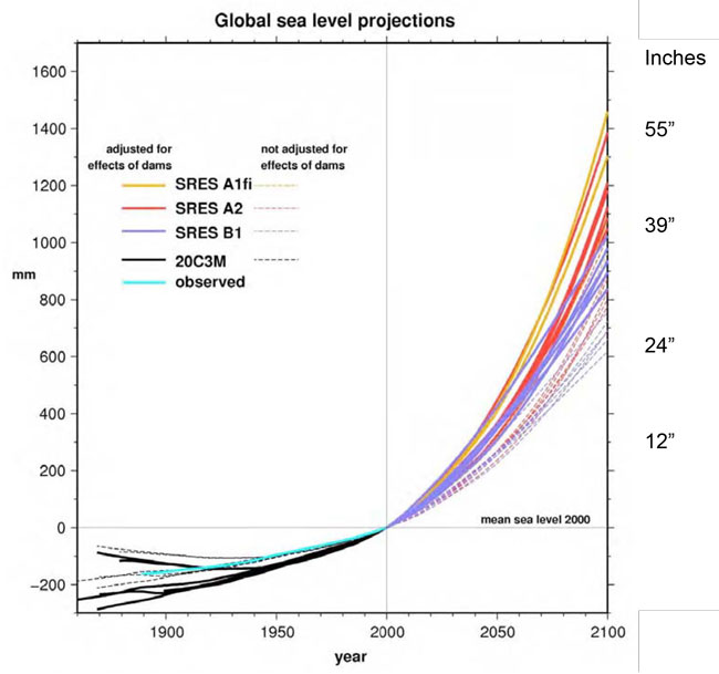
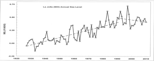
The results of the three simulation scenarios indicate sea-level increases of 12 to 18 inches (30 to 45 cm) by 2050. Projected SLR based on the application of the Rahmstorf 2007 method with and without adjustment for the effects of dams are compared with observed values between 1900 and 2000. These projections are shown in Figure 3-4.
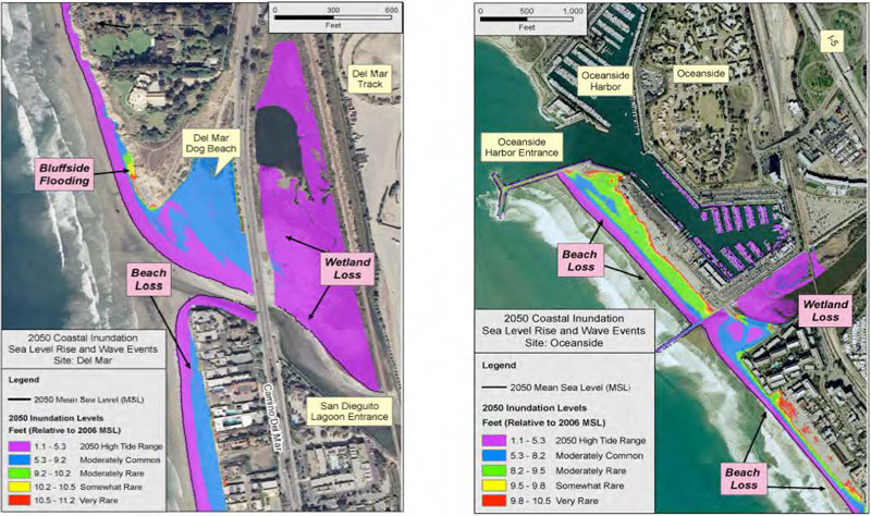
The study combined the effects of SLR, tidal fluctuations and run-up from moderately common wave events (from SIO's Coastal Data Information Program, or CDIP) to produce inundation maps for six flood-prone areas in the region (i.e., Oceanside, Del Mar, La Jolla Shores, Mission Beach, Coronado, and South Imperial Beach). The graphics show inundation areas in the year 2050 under the following frequency categories and can be seen at (http://www.cleantechsandiego.org/):
- Very Likely: predicted high tide range in 2050
- Moderately Common: estimated sea level + tide + wave run-up elevation recurrence, on average, every five years in the 50-year simulation. Expected to occur every few years when El Niño conditions are not present.
- Moderately Rare: estimated sea level + tide + wave run-up elevation recurrence, on average, every 10 years in the 50-year simulation; but expected in most years when El Niño conditions are present.
- Somewhat Rare: estimated sea level + tide + wave run-up elevation recurrence on average every 25 years, based on the 50-year simulation.
- Very rare: the highest combination of sea-level + tides + wave run-up elevation in the 50-year simulation.
An example inundation simulation is shown in Figure 3-5 for the Cities of Del Mar and Oceanside shoreline. As the decades proceed, the simulations show an increasing tendency for heightened sea level events to persist for more hours, which would likely cause greater coastal erosion and related damage.
3.4.2 The Impacts of Sea Level Rise on the California Coast (Heberger et al. 2009)
California Energy Commission's Public Interest Energy Research (PIER) Program established the CCCC to document climate change research relevant to the State. This center is a virtual organization with core research activities at SIO and the University of California, Berkeley, complemented by efforts at other research institutions. This study is a part of a report series that details ongoing Center-sponsored research.
The report cites recent research by leading climate scientists who claimed that more accurate sea level measurements by satellites indicate that SLR from 1993 to 2006 has outpaced the IPCC projections at some locations (Rahmstorf 2007). The authors suggest that the climate system, particularly sea levels, may be responding to climate changes more quickly than the models predict. Additionally, most climate models fail to include ice melt contributions from the Greenland and Antarctic ice sheets and may underestimate the change in volume of the world's oceans.
To address these new factors, the PIER projects used SLR forecasts developed by a team at the SIO led by Dr. Dan Cayan. Using a methodology developed by Rahmstorf (2007), Cayan et al. (2009) produced global sea level estimates based on projected surface air temperatures from global climate simulations for both the IPCC A2 and B1 scenarios using the output from six global climate models:
- the National Center for Atmospheric Research (NCAR) Parallel Climate Model;
- the National Oceanic and Atmospheric Administration (NOAA) Geophysical Fluids Dynamics Laboratory version 2.1;
- the NCAR Community Climate System Model (CCSM);
- the Max Planck Institute ECHAM3;
- the MIROC 3.2 medium-resolution model from the Center for Climate System Research of the University of Tokyo and collaborators, and
- the French Centre National de Recherches Meteorologiques models.
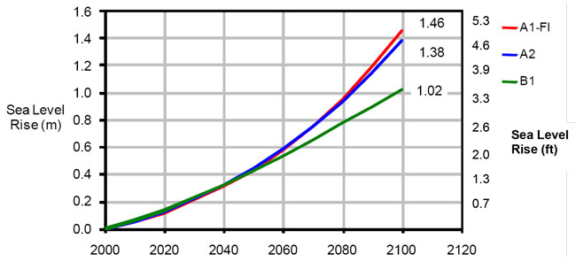
Additionally, Cayan et al. (2009) modified the SLR estimates to account for water trapped in dams and reservoirs that artificially reduced runoff into the oceans (Chao et al. 2008). Absolute SLR along the California coast was assumed to be the same as the global estimate. Based on these methods, Cayan et al. (2009) estimate an overall projected rise in MSL along the California coast for the B1 and A2 scenarios of 39 inches (1.0 meter) and 55 inches (1.4 meters), respectively, by 2100. The more severe A1FI scenario, which assumes continued high-level use of fossil fuels, was not used in this analysis but is shown in Figure 3-6 for comparison.
3.4.3 Climate Change-Related Impacts in the San Diego Region by 2050 (Messner et al. 2009)
This study states that it relies heavily on research conducted in the Focus 2050 Study to analyze climate and SLR impacts to the San Diego region in the year 2050. The report's analysis and conclusions, in regard to SLR, appear identical to those of the prior study (Messner et al. 2009).
3.4.4 Climate Action Strategy (SANDAG 2010)
SANDAG's CAS is a planning-level document that serves to help policymakers address climate change as they make decisions to meet the needs of a growing population, maintain and enhance the quality of life, and promote economic stability. The document outlines goals and objectives to work toward that end and specifically addresses SLR under Goal 4 and Objective 4b as listed in the Introduction to this study.
3.4.5 Sea Level Rise Adaptation Strategy for San Diego Bay (ICLEI 2012)
The Adaptation Strategy document is intended to provide participating steering committee jurisdictions with policy recommendations that will aid in making bay-front communities more resilient to SLR and its associated impacts such as coastal flooding, erosion, and ecosystem shifts. The steering committee consists of staff from the:
- City of Chula Vista;
- City of Coronado;
- City of Imperial Beach;
- City of National City;
- City of San Diego;
- Port of San Diego;
- San Diego County Airport Authority; and
- International Council for Local Environmental Initiatives.
The bay was separated into a number of different potentially impacted sectors (i.e., ecosystems, facilities, stormwater/wastewater systems, etc.) for which vulnerabilities and adaptation strategies were developed. Impacts were evaluated from four SLR planning scenarios, as follows:
- 2050 Daily Conditions — Mean high tide in 2050 with 0.8 feet (0.5 meters) of SLR.
- 2050 Extreme Event – 100‐year extreme high water event in 2050, with 0.8 feet (0.5 meters) meters of SLR, including such factors as El Niño, storm surge, and unusually high tides.
- 2100 Daily Conditions – Mean high tide in 2100 with 4.9 feet (1.5 meters) of SLR.
- 2100 Extreme Event – 100‐year extreme high water event in 2100, with 4.9 feet (1.5 meters) of SLR, including such factors as El Niño, storm surge, and unusually high tides.
3.5 Scientific Publications
A number of scientific publications were the basis of the SLR scenarios. These scenarios were the foundation of the previously discussed guidance documents. Relevant scientific publications are summarized in this section.
3.5.1 Rahmstorf (2007)
A semi-empirical approach has been developed by Stefan Rahmstorf of the Potsdam Institute for Climate Impact Research, Germany, in an attempt to address the IPCC model limitations. The approach uses existing temperature projections while using a linear model based on observations from 1880 to 2001 to predict SLR directly from temperature changes. It may capture the effect of mechanisms such as the loss of mass from ice caps, which may already be occurring but which are not yet understood in detail. The semi-empirical approach describes SLR from 1990 to 2006 better than the TAR, although it has not been compared to the 4AR. The approach is controversial in its application of statistical methods but has been widely quoted and is regularly used in planning literature. It increases the estimate of 21st Century SLR to between 1.6 to 4.6 feet (50 and 140 cm) between 1990 and 2100.
3.5.2 Vermeer & Rahmstorf (2009)
In 2009, the semi-empirical relationship for projecting SLR was revised to account for second-order warming effects, which result in quicker temperature changes (Vermeer and Rahmstorf 2009). A second term was added to the relationship to account for shorter time-scale sea-level responses such as heat content in the ocean surface. The updated relationship was found to capture short-term variability when utilized with global climate change models that could account for solar variability, volcanic activity, changes in greenhouse gas concentration, and tropospheric sulfate aerosols. The revised relationship resulted in higher SLR projections for the same IPCC scenarios used in the Rahmstorf 2007 study. The revised SLR projections ranged from 2.66 to 5.87 feet (0.81 to 1.79 meters) above 1990 levels by the year 2100, as summarized in Table 3-4.
Table 3-4. Vermeer and Rahmstorf (2009) Sea Level Rise Projections to Year 2100
| Scenario | Emissions Categories | Sea-level Rise feet (meters) |
|---|---|---|
| B1 | Low to Medium-Low | 2.66 – 4.30 (0.81 – 1.31) |
| A1T | Low to Medium-Low | 3.18 – 5.18 (0.97 – 1.58) |
| B2 | Medium-Low to Medium-High | 2.92 – 4.76 (0.89 – 1.45) |
| A1B | Medium-Low to High | 3.18 – 5.12 (0.97 – 1.56) |
| A2 | Medium-Low to High | 3.22 – 5.09 (0.98 – 1.55) |
| A1FI | High | 3.71 – 5.87 (1.13 – 1.79) |
3.5.3 Houston and Dean (2011)
The study titled, Sea-Level Acceleration Based on U.S. Tide Gauges and Extensions of Previous Global Gauge Estimates (Houston & Dean 2011), analyzes the U.S. and global tide gauge data with durations of 60 to 156 years, starting in the Year 1930 to 2010. Based on this data set, the study found that empirical-based SLR predictions postulated by IPCC, Rahmstorf, and others were not observed in the long-term tide gauges, and many of them showed small average SLR decelerations. The study uses these findings to question the acceleration of SLR that has been cited in most model projections (e.g., Vermeer & Rahmstorf 2009). The study states that without the empirical-based predictions for SLR acceleration, the 20th Century SLR trend of 0.7 inches/year (1.7 mm / year) would produce a rise of only approximately 0.5 feet (0.15 m) from 2010 to 2100. The study also poses the question of why the increase in global temperatures of 1.33°F (0.74°C) during this period did not result in the acceleration of rising sea levels, and a deceleration occurred over certain periods.
3.5.4 Rahmstorf and Vermeer (2011)
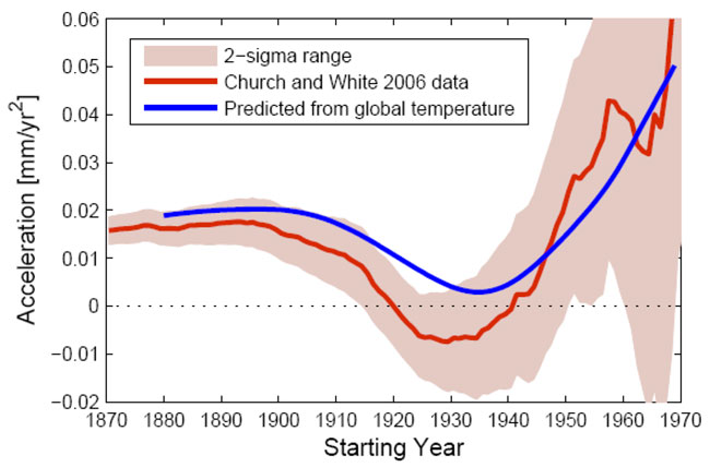
As a rebuttal to Houston & Dean (2011), Rahmstorf and Vermeer published Discussion of: Houston, J.R. and Dean, R.G., 2011. Sea-Level Acceleration Based on U.S. Tide Gauges and Extensions of Previous Global-Gauge Analyses. The paper demonstrates that the results of the Houston & Dean (2011) study are the result of their specific focus on acceleration since the year 1930, which represents a unique minimum in the acceleration curve (Figure 3-7). Further, the study suggests that global SLR is accelerating in a way that is strongly correlated with global temperature and that this correlation explains the acceleration minimum for periods starting around 1930 as being due to the mid-twentieth-century plateau in global temperature.
4.0 Guidance from Funding Agencies
Many agencies provide funding for transportation projects being administered by SANDAG, Caltrans, and coastal cities. The railway improvements in the LOSSAN Corridor are being funded by FRA, FTA, the State of California, Caltrans Division of Rail, Amtrak, and the local TransNet Program. The freeway projects along the North County Coastal Corridor are funded by FHWA, Caltrans, the State of California, and the local TransNet Program. The funding agencies were contacted to obtain their current guidance on SLR. This section summarizes guidance from these agencies.
4.1 Federal Funding Agencies
4.1.1 Federal Rail Authority
The FRA and the FTA are divisions within the USDOT. The FRA promulgates and enforces rail safety regulations, administers railroad assistance programs, conducts research and development in support of improved railroad safety and national rail transportation policy, provides for the rehabilitation of Northeast Corridor rail passenger service, and consolidates government support of rail transportation activities.
The FRA does not have specific SLR guidance; therefore, USDOT guidance would apply (EIC 2011). This guidance is summarized in Section 1.0 of this document. Adherence of the project to this guidance would require the incorporation of climate change adaptation strategies.
4.1.2 FHWA
As discussed in section 3.2.4, the FHWA does not currently require consideration of SLR in bridge project designs. As previously stated, guidance for bridge design is published in HECs and SLR is discussed in HEC-25 (Douglass and Krolak 2008).
4.2 State Transportation Agencies
4.2.1 Caltrans Division of Rail
The Caltrans Division of Rail follows the 2013 State Guidance on SLR. This agency is a member of CO-CAT and operates according to the guidelines developed by the State.
4.2.2 Caltrans Highways
Caltrans has a process, described in Section 3.3.8 of this document whereby projects are analyzed in light of future SLR. Caltrans takes prediction values shown in Table 3-4 of this document and considers the project's potential effect from SLR, and analyzes and designs accordingly. SLR values considered are those of the State's guidance document from 2013.
4.2.3 Amtrak
Amtrak is the business name for the National Railroad Passenger Corporation, a government-owned passenger Rail Corporation. Amtrak does not have any specific guidance on SLR. However, rail projects bordering the coast are evaluated on a case-by-case basis taking into account all pertinent design parameters. Coastal protection is provided to rail infrastructure based on geography/topography, site-specific conditions, historical information, and a risk assessment of future impacts (Richter 2012).
4.3 Local Agencies
SANDAG is developing this study to provide local guidance for transportation projects. Some local coastal agencies are preparing/have prepared plans that address climate change and SLR, as detailed in Table 4-1.
Table 4-1. San Diego Coastal Cities Preparing SLR Guidance Plans
| City | Document Title | Author | Status |
|---|---|---|---|
| Oceanside | None | N/A | N/A |
| Carlsbad | None | N/A | N/A |
| Encinitas | Climate Action Plan | City of Encinitas | Complete |
| Solana Beach | Local Coastal Plan Policy, Chapter 4 (Natural Hazards) | City of Solana Beach | Complete |
| Del Mar | None | N/A | N/A |
| City of Chula Vista City of Coronado City of Imperial Beach City of National City City of San Diego Port of San Diego San Diego County Airport Authority |
SLR Adaptation Strategy San Diego Bay | ICLEI et.al. 2012 | Complete |
5.0 Sea Level Elevations
Review and analyses of federal, state, and local SLR studies and other literature summarized herein provide potential future SLR scenarios for the purposes of planning and engineering design of the Project. The results of this technical review are presented in this section.
5.1 Historical Global Sea Level Rise
The latest assessment of global historic SLR estimates provided by NRC 2012 gives the following measured rates:
- Long-term (past 50 to 100 years) rates of about 0.07 inches/year (1.8 mm / year), as estimated from tide gages; and
- Recent (post-1990) rates of about 0.13 inches/year (3.2 mm / year), as estimated from satellite altimetry and tide gauges.
These rates are in close agreement with the 4AR and provide a context for projected rates into the future.
5.2 Local Sea Level Rise
As previously mentioned, the rate of global SLR is of less practical importance than the local rate of SLR relative to the land. The first analysis method of the local conditions is to look to long-term tide gauge records in the Project area. There are two long-term water level records within the study area (La Jolla and San Diego Bay) operated by NOAA. An analysis of the components of relative SLR is presented in this section, which includes analysis of local tide gage data as well as the vertical movement of the land over this same period.
5.2.1 Tide Gage Data
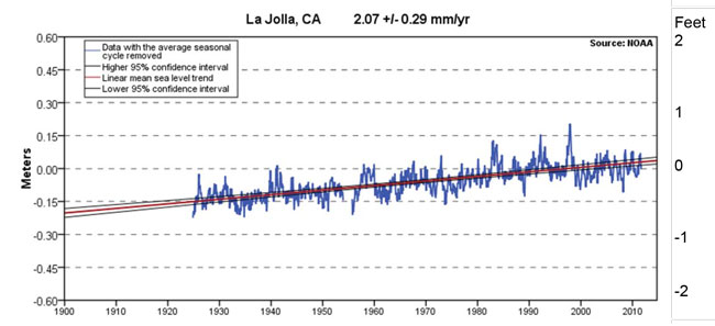
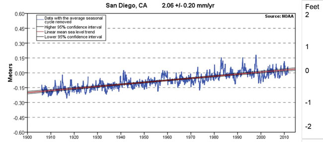
NOAA estimates the rate of local SLR at the La Jolla gage as 0.08±0.01 inches/year (2.07±0.29 mm / year, 0.68±0.1 feet (0.21 meter/century), based on monthly MSL from 1924 to 2006 (NOAA 2012). This is generally consistent with the global rate (i.e., 0.07 inch/year; 1.7 mm / year), suggesting that uplift or subsidence is not contributing significantly to the rate of local SLR at the Project site. Similarly, NOAA has analyzed the tidal record for San Diego Bay and estimates the rate of local SLR as 0.08±0.01 inches/year (2.06±0.20 mm / year, 0.68 feet 0.21 meter/century), based on monthly MSL from 1906 to 2006. Figure 5-1 and Figure 5-2 show these water level records.
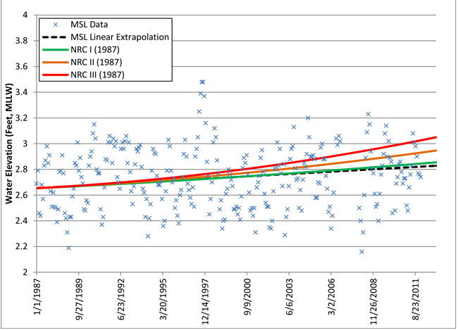
Local SLR was compared to the NRC 1987 projections to determine how the region was performing over the last 30 years (Figure 5-3). Based on this tidal record, the region appears to be following the low SLR projection (NRC I). As shown in this graphic, from 1987 through 2010, MSL recorded at the La Jolla tide gage followed the NRC I projection closely and fell below the high projection (NRC III) by approximately 0.2 feet. This analysis should be considered a first-order estimate and a more detailed analysis would be necessary to reach any firm conclusions.
5.2.2 Vertical Land Movement
Vertical land movement in the San Diego region depends on varying contributions of glacial isostatic adjustment, sediment compaction, fluid withdrawal or recharge, and local compressional tectonics that may or may not be related to earthquake faults. Two very different assessments of the vertical land movement have been made for the San Diego region and both are presented below. Although they vary, the magnitude of the vertical land changes does not significantly affect SLR because this is typified primarily by strike-slip (lateral) movement rather than vertical movement.
The NRC report (2012) found that the San Diego region is projected to subside at a rate of 0.06 inch/year (1.5 mm/ year) from 2010 to 2100 based on projections from existing satellite records. This subsidence rate was accounted for in the NRC 2012 SLR projections.
In contrast, Abbott (1999) indicates that land in the San Diego region is slowly being uplifted as presented in the book titled The Rise and Fall of San Diego, 150 Million Years of History Recorded in Sedimentary Rocks. This book states that the land is rising at an average rate of about 5.5 inches (14 cm) per thousand years or 0.55 inches per century. In the last 80,000 years the rate of uplift seems to have increased to nearly 12 inches (30.5 cm) per thousand years (1.2 inches per century); southwest of the Rose Canyon fault, the uplift rate is closer to 18 inches (45.7 cm) per thousand years (1.8 inches per century). This equates to an uplift rate of 0.01 to 0.02 inches (0.03 to 0.05 cm) per year. Since this uplift value is approximately equal to the SLR measurement errors and is well within the SLR variability based on different projections, this uplift rate can be ignored and not applied to the global SLR rate to determine the local SLR in the San Diego region. Consequently, at this time, local uplift does not appear to be a significant factor in assessing local relative SLR rates in the region.
5.2.3 Recent Observations
Recently the rate of SLR along the California coast (and the west coast of North and Central America as a whole) has slowed or even reversed (Bromirski et al. 2011). The following studies support this observation.
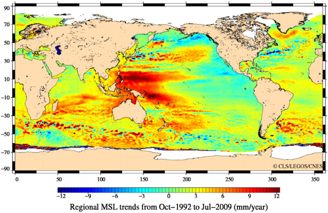
- Based on multi-satellite altimetry (Cazenave et al. 2008; CNES et al. 2010) and tide gauge records (Bromirski et al. 2011; Coastal Environments 2010), the sea level along the Southern California coast has dropped, as shown in Figure 5-4.
- Based on monthly mean water levels measured at La Jolla (Willis et al. 2008), the rate of sea-level increase between 1993 and the end of 2009 was only 0.02 inches (0.6 mm) per year (0.2 feet (6.1 cm) per century) – much less than the 20th Century average.
A localized decrease in ocean temperatures and hemispheric wind stress patterns appear to be responsible for this slowing or reversal in sea level along with the Pacific Coast of North America (Cazenave et al. 2008; Bromirski et al. 2011). Figure 5-5 shows global sea surface temperatures, and those for the eastern Pacific Ocean are lower than those for the central and western Pacific. Recent changes in the wind stress patterns may indicate a regime shift toward conditions allowing SLR to resume at rates equal to or greater than global rates.
5.3 Tidal Range Increase
The tidal range measured at La Jolla has increased measurably during the 20th Century. This means, for example, that the elevation of Mean Higher High Water (MHHW) is rising more rapidly than the MSL (Flick et al. 2003). Based on measurements at La Jolla from 1924 to 2006, the rate of SLR at the MHHW datum is approximately 0.74 feet (22 cm) per century, compared to 0.66±0.10 feet (20 cm ± 3 cm) per century at MSL and 0.66 feet (20 cm) per century at Mean Lower Low Water (MLLW).
The mechanisms causing this increase in the tidal range are not known, and it is also not known whether the rate of increase will increase, decrease, or remain constant. The difference between the two rates of increase – 0.66 feet (20.7 cm) per century at MSL versus 0.74 feet (22.5 cm) per century at MHHW – is small compared to the general level of uncertainty regarding the future SLR. Consequently, it does not seem necessary to account for the increase in tidal range in most planning activities.
6.0 Recommended Sea Level Rise Scenarios
Since funding is possible from both state and federal entities, it is recommended that the Interim Guidance (2010) and USACE (2011) guidance be followed for SLR in the planning and design for this Project. However, the most recent guidance from CO-CAT (2013) with scientific input from the OPC should also be considered as it represents the most recent science. Since the Program will be constructed in phases, SLR rates are given for a number of planning horizon years below for consideration of the various capital improvement projects. Projects conducted under the NCC Program that are planned for design and construction in later years (e.g., beyond the year 2020) should consider the relevant SLR projections and agency guidance available at that time. This could also be addressed through continued updating of this document and subsequent use of the information for future planning and design of NCC Program projects.
6.1 Concurrence with State of California Guidance
SLR scenarios were extracted from CO-CAT State Guidance (2013) for the various planning horizon years, as shown in Table 6-1.
Table 6-1. State of California Sea Level Rise Scenarios (CO-CAT Guidance 2013)
| Year | Low Inches (cm) | High Inches (cm) |
|---|---|---|
| 2030 | 1.56 (3.92)** | 11.76 (29.87)*** |
| 2050 | 4.68 (11.89)** | 24.00 (60.96)*** |
| 2100 | 16.56 (42.06) | 65.76 (167.03) |
6.2 Concurrence with USACE (2011) Guidance
Assuming the Project requires a USACE permit and/or involves federal funding, SLR scenarios were generated for the Project consistent with USACE (2011) guidance. These scenarios are shown in Table 6-2 and presented graphically in Figure 6-1 for horizon years 2030, 2050, and 2100.
Table 6-2. Sea Level Rise Scenarios Per USACE (2011) Guidance
| Year | Low Rate (Linear Extrapolation) Inches |
Low Rate (Linear Extrapolation) Centimeters |
Intermediate Rate (NRC I) Inches |
Intermediate Rate (NRC I) Centimeters |
High Rate (NRC III) Inches |
High Rate (NRC III) Centimeters |
|---|---|---|---|---|---|---|
| 2030 | 1.20 | 3.05 | 3.60 | 9.14 | 8.40 | 21.34 |
| 2050 | 3.60 | 9.14 | 7.20 | 18.29 | 19.20 | 48.77 |
| 2100 | 7.20 | 18.29 | 19.20 | 48.77 | 58.80 | 149.35 |
6.3 Sea Level Rise Guidance Discussion
The State and Federal guidance presented above differs most notably as years progress toward 2100. The recommended approach for each PDT is to consider the full range of projected SLR scenarios over the design life of the Project and, if possible, design to accommodate the highest prediction. The full range of SLR should be 16.56 inches (1.4 feet) to 65.76 inches (5.5 feet) from 2000 to 2100 per State guidance (March 2013 CO-CAT). Should conflicting design requirements limit the PDT from designing to the highest projection of 5.5 feet, then a lower value for SLR, based on risk tolerance assessment or planned adaptation strategies for the structures, should be considered. That lower level of SLR to be considered is to be determined based on project-specific requirements and constraints. Adaptation strategies are discussed in more detail in Section 8.0. In addition, even in cases where design requirements do not limit the ability to design for the highest prediction, the PDT might consider conducting an economic analysis to determine if it is more cost-effective to develop designs based on lower projections with adaptation measures. Alternatively, risk tolerance considerations of the impacts on public health and safety, public investments, and the environment may support the use of lower SLR projection for the project design process.
7.0 Design Water Level Guidance
Most bridge structures are built across rivers, streams, and creeks that are dominated by fluvial (riverine) processes while some are built across large estuaries that are dominated by ocean (tidal) processes. The NCC Program bridges will cross rivers and lagoons that are dominated by ocean processes throughout dry periods and fluvial processes during wet periods. Consequently, the water levels that should be considered in the design of the NCC Program corridor bridges should include consideration of these two primary water level components: Ocean Water Level and Fluvial Water Level. These two water level components are described in this section.
Before discussing these components, it is important to define the vertical datum that is used as a reference for such discussions. Section 7.1, defines the vertical datum used in this section along with the corresponding rationale for its use. This section further defines components of ocean water level (Section 7.2), extreme water levels (Section 7.3), fluvial water levels (Section 7.4), and combined water levels (Section 7.5).
7.1 Vertical Datums
Several vertical datums are used for surveys and structure designs within the coastal zone. Elevations presented herein are relative to the National Geodetic Vertical Datum of 1929 (NGVD 29) to be consistent with the historical datum used thus far for the San Diego Region LOSSAN bridges (Smith 2012). However, all four of the common vertical datums (NGVD 29, NAVD 88, MLLW, and MSL) are used in this study for ease of reference to source documents. The relationship of the first three of these vertical datums to NGVD 29, as well as to one another at the Scripps Pier in La Jolla is shown in Figure 7-1. The water level information presented in Figure 7-1 is based on the National Tidal Datum Epoch of 1983 - 2001.
7.2 Ocean Water Level
Ocean water levels are influenced by several components that occur over different time and spatial scales. The major components of ocean water levels, which are listed below, are discussed in more detail herein.
- Astronomical tide;
- Storm surge;
- Wave set-up;
- Cyclic climatic patterns (e.g., El Niño Southern Oscillation/ENSO);
- Tsunamis; and
- Local SLR.
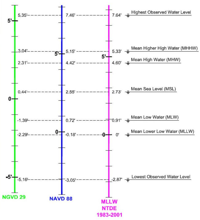
To obtain quantitative information on the ocean water level components listed above, NOAA conducts ocean water level measurements at numerous tide gauge locations (stations) throughout the U.S., including Southern California. The NOAA station closest to the LOSSAN corridor is located at Scripps Pier in La Jolla. Given that this gage station is located on the open coast, the water levels measured at this station include all of the ocean water level components discussed above, although it may not obtain the maximum value of wave set-up since wave set-up varies with a location offshore. The tidal datums, developed by NOAA through analysis of the ocean water level measurements collected at this gage station, are presented in Table 7-1. As seen in the table, the highest water level observed at the Scripps Pier reached 5.36 feet, NGVD29 on November 13, 1997.
Table 7-1. Tidal Datums for La Jolla (Based on 1983-2001 Tidal Epoch)
| Description | Elevation (ft, MLLW) | Elevation (ft, NGVD 29) | Elevation (ft, MSL) | Elevation (ft, NAVD 88) |
|---|---|---|---|---|
| Extreme High Water (11/13/1997) | 7.65 | 5.36 | 4.92 | 7.47 |
| Mean Higher High Water (MHHW) | 5.33 | 3.04 | 2.60 | 5.15 |
| Mean High Water (MHW) | 4.60 | 2.31 | 1.87 | 4.42 |
| Mean Tidal Level (MTL) | 2.75 | 0.46 | 0.02 | 2.57 |
| Mean Sea Level (MSL) | 2.73 | 0.44 | 0.00 |
2.55 |
| National Geodetic Vertical Datum 1929 (NGVD 29) | 2.19 | 0.00 | -0.44 | 2.11 |
| Mean Low Water (MLW) | 0.90 | -1.39 | -1.83 | 0.72 |
| North America Vertical Datum 1988 (NAVD 88) | 0.18 | -2.11 | -2.55 | 0.00 |
| Mean Lower Low Water (MLLW) | 0.00 | -2.29 | -2.73 | -0.18 |
| Extreme Low Water (12/17/33) | -2.87 | -5.16 | -5.60 | -3.05 |
7.2.1 Astronomical Tide
The astronomical tides, which are driven by the gravitational influence of the celestial bodies on the Earth's oceans, represent the most persistent component of ocean water levels. The tides in Southern California are semi-diurnal (two high tides and two low tides each day) with a diurnal inequality (one higher high water and one lower high water as well as one lower low water and one higher low water). Due to the relative position of the three celestial bodies with the greatest influence on the tides (Earth, Sun, and Moon), the tides include two neap tides and two spring tides each month. The neap tides, which occur when the Earth, Sun, and Moon are out of alignment, are relatively small in magnitude. Tides that are relatively large in magnitude, known as spring tides, occur when the Earth, Sun, and Moon are in alignment.
7.2.2 Storm Surge
Storm surge is the increase in ocean water level caused by the decrease in air pressure (i.e., barometric pressure) associated with a storm, plus the increase in ocean water level caused by wind (i.e., wind set-up) blowing across the ocean water surface. Storm surge can be quite large (e.g., 10 to 20 feet) in areas with large storm events and extensive, relatively shallow continental shelves (e.g., Gulf of Mexico coast). In Southern California, the continental shelf is relatively narrow and such large storm events (e.g., tropical cyclones) rarely occur in the nearshore waters. As described below, the two reasons why tropical cyclones rarely occur in Southern California are due to relatively low sea surface temperatures and the usual upper-level winds in the eastern Pacific.
- Sea Surface Temperature: The tropical cyclones draw fuel from heat stored in the upper ocean. Typically, ocean surface waters of 80 degrees Fahrenheit are required to form and fuel tropical cyclones. But water temperatures never get that high in the coastal waters of California. On rare occasions, they may reach about 75 degrees Fahrenheit near the shore in Southern California, typically during an El Niño episode. But generally speaking, low 60s is about as warm as they get farther from shore and elsewhere in coastal California according to an article published on the Jet Propulsion Laboratory (JPL 2012) web site. Global warming has raised the average ocean temperature by 0.18 degrees Fahrenheit over the century (National Geographic 2012).
- Upper-Level Winds: The upper-level winds in the Tropics tend to carry and steer storms to the west and northwest, away from the coast, and also tend to shear the tops off of tropical cyclones and break them apart. Lower-level winds off Southern California are prevailing northwest sea breezes. These prevailing northwesterly winds push warmer surface waters offshore, drawing cooler subsurface waters up to the surface, and this further adds to the cool nature of the nearby ocean waters that tend to weaken any cyclones that approach California.
Historically, there has never been a documented case of a hurricane making landfall in California, although California has been affected by a few tropical cyclones which occurred in El Niño years around September. In Southern California, the primary threat from tropical cyclones is not winded or storm surge, but, rather, rainfall which has led to flooding damage and occasionally, causalities. Below are a few notable tropical cyclones that affected Southern California in recorded history. - The San Diego hurricane of 1858. This is the only tropical cyclone ever known to have affected California as a hurricane. The storm formed in the eastern Pacific Ocean in late September and intensified into an estimated Category 1 hurricane with estimated highest winds of about 85 miles per hour (74 knots). By October 2, its untypical north-northeasterly course had steered it just off the coast of San Diego, where cooler waters and strong wind shear weakened it slightly. Luckily, just before it was about to make landfall, the storm made a turn to the west-northwest and then dissipated near Santa Catalina Island. Despite the near-miss, instrument records in San Diego indicate the area experienced a hurricane or near-hurricane force winds of approximately 75 mph (65 knots), heavy rain, and considerable property damage. Researchers reported that based upon historical records and modeling results, such a storm can be expected in the San Diego area about every 200 years, most likely during an El Niño event.
- The Tropical Cyclones of the El Niño of 1938-39. In September 1939, Southern Californians experienced the first of four tropical cyclones affecting the region during the El Niño of 1938-39. The first two storms - remnants of hurricanes - tracked northeastward across northern Baja California into southwest Arizona, bringing heavy rainfall to parts of Southern California: up to 7 inches for the first storm and up to 4 inches for the second. A third storm dissipated in southern Baja California but brought up to 3 inches of rain to parts of the Southland. Then, on Sept. 25, an unnamed storm made landfall near San Pedro with winds near 50 mph (43 knots), becoming the only tropical cyclone to ever make landfall in Southern California as a tropical storm in recorded history. In addition to the winds, the storm brought up to 5 inches (13 centimeters) of rain to the Los Angeles basin and as much as 12 inches (30 centimeters) of rain to the surrounding mountains. The storm caused heavy flooding and killed at least 45 people, mostly at sea. Low-lying coastal regions from Malibu to Huntington Beach were flooded, and thousands of people were stranded in their homes. There was heavy street flooding - up to 3 feet (1 meter) in places. The fact that the storm came on suddenly, leaving many people unprepared, led to the establishment of a Southern California forecast office for the United States Weather Bureau in 1940.
- Hurricane Kathleen occurred in mid-September of 1976 during an El Niño year. It made landfall in northern Baja California and moved into California and Arizona, still at tropical storm strength. Sustained winds of 57 mph were reported in Yuma, Ariz. The storm brought 6 to 12 inches of rain to Southern California's central and southern mountains. Ocotillo, California suffered catastrophic damage, with 70 to 80 percent of the town destroyed. Twelve deaths were blamed on the storm in the United States. The Associated Press reported hundreds of homes were destroyed or damaged in the United States by Kathleen, which was described as a one-in-160-year event.
- Hurricane Linda occurred in September 1997 during an El Niño year. It is the strongest eastern Pacific hurricane on record. This Category 5 hurricane at one point had maximum sustained winds of 185 mph (161 knots). For a couple of days, National Hurricane Center forecasters warned the storm could barrel into Southern California, most likely as a tropical storm. Fortunately, the storm turned westward away from land. Still, Linda brought significant rainfall across parts of Southern California and waves up to 18 feet, and caused several million dollars in property damage.
- Hurricane Nora happened in September 1997 during an El Niño year. In the wake of Hurricane Linda, Hurricane Nora crossed into California and Arizona from Baja California as a tropical storm, bringing heavy rains to parts of southeast California and Arizona. The storm caused hundreds of millions of dollars in damage, especially to agriculture.
7.2.3 Wave Set-up
Wave set up is the increase in ocean water level associated with the excess momentum caused by breaking waves. Wave set-up can exceed one foot in Southern California during events with large waves. Although wave set-up can contribute to the overall ocean water level, the effect is limited to the breaker zone and beach area. Therefore, locations farther inland are generally not impacted by wave set-up.
7.2.4 Cyclic Climatic Patterns
Cyclic climatic oscillations can have a large impact on ocean water levels with this impact extending over large temporal and spatial scales. The two largest cyclic climatic oscillations are the El Niño Southern Oscillation (ENSO) and the Pacific Decadal Oscillation (PDO). ENSO occurs every four to seven years and causes an increase in the ocean water level of the west coast of North and South America. It is common for ENSO events to raise the ocean water level by 0.5 to 1.0 foot. For example, during the 19971998 ENSO event, monthly MSLs in southern California were increased by up to 1.0 foot (USACE 2002). Local tide gauges recorded up to 8.6 inches of water level increase for the same event. On a longer time scale, the PDO was recently shown to be a likely cause of suppressed ocean water levels on the West Coast of North America and may lead to a rapid increase in local ocean water levels in the near future (Bromirski 2011).
7.2.5 Tsunamis
Tsunamis are typically caused by submarine earthquakes and landslides. They are a long period, fast-moving waves generated by large displacements of the seafloor (e.g., underwater earthquakes or landslides) or impacts from celestial bodies (e.g., meteors). Earthquake faults along colliding tectonic plates tend to be thrust faults that result in vertical land movement and ocean water displacement. These faults occur along the western Pacific Ocean near Asia and the Eastern Pacific along Alaska and South America. California is located along a boundary of sliding tectonic plates called strike-slip faults. The San Andreas Fault separates two plates with the one west of the fault moving north, and the plate east of the fault moving south. Strike-slip faults do not generally result in tsunamis unless they cause submarine landslides. Figure 7-2 shows the San Andreas earthquake fault in California.
The tsunami generated by the Miyagi earthquake in Japan on April 7, 2011, reached Southern California with a very small tsunami wave (less than a foot) observed along the coast. A more pronounced tsunami wave was recorded after the Chile earthquake on February 27, 2010, where waves of approximately two feet were measured at San Diego. There have been several historical tsunamis of significant magnitude along the Southern California coast generated by seismic events in Alaska and Chile. A number of references were reviewed relative to the potential tsunami wave heights within the Project area and this information is summarized below.
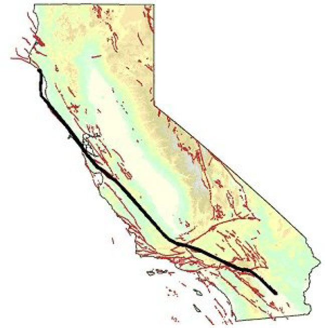
7.2.5.1 State of California Tsunami Inundation Maps (2009)
The "Tsunami Inundation Maps for Emergency Planning" were published on June 1, 2009, through a joint effort by the State of California Office of Emergency Services, the California Geologic Survey, the University of Southern California Tsunami Research Center, and NOAA. The maps present the impacts of both local and distant sources of tsunamis on the California coastline. Tsunami inundation areas were depicted on these maps based on the assumption that the tsunami occurred during mean high water. The maps represent the maximum tsunami run-up from a number of credible, extreme, tsunami sources. The maps do not represent inundation from a single event; rather they display the maximum tsunami inundation generated from either a local or distant source event affecting a given region. This combination of the mean high water level and worst-case scenario tsunami event was used to create what was called a "credible upper bound" for each region of the coastline for the main purpose of emergency preparedness, as opposed to providing design guidance or criteria. Since the maps represent the worst-case model results for each portion of the coastline, specific water level elevations associated with the tsunami inundation areas were not given. The recurrence interval of the events characterized by the California Geology Survey maps is not provided. Researchers associated with the map study indicate that they are likely on the order of 1 in every 2,500 years (Dykstra 2012).
7.2.5.2 SONGS Tsunami Study (2011)
The study updated the San Onofre Nuclear Generating Station (SONGS) tsunami hazard analysis and found that the new maximum tsunami height is approximately 19.9 to 22.9 feet MLLW (17.6 to 20.6 NGVD29) (SCE 2011). The study utilized the State of California Tsunami Inundation Maps (2009) with a slight modification to account for the maps' exclusion of a seawall that fronts a portion of the SONGS facility. As mentioned above, the State's modeling effort is considered conservative in that its objective was to provide a "credible upper bound" of tsunami inundation at any location along the coastline for the main purpose of emergency preparedness and not necessarily for design criteria.
7.2.5.3 Ports of Long Beach and Los Angeles Tsunami Study (2007)
The Ports of Long Beach and Los Angeles (POLA/POLB) completed a study in 2007 of potential exposure to tsunamis to identify concerns. The study utilized a Boussinesq wave model to simulate tsunami wave propagation into the POLA/POLB. Seven potential tsunami sources were modeled, including four local tectonic scenarios, two local submarine landslide scenarios, and one distant tsunami source scenario. Model results suggest the worst-case scenario tsunami for the region would be from a landslide in the vicinity of Palos Verdes. This tsunami could result in water levels in excess of 23 feet and current speeds up to 8.2 feet /second in some locations. Regarding the frequency of occurrence, the study found that based on the seismicity, geodetics, and geology of the region, a large locally-generated tsunami from either local seismic activity or a local submarine landslide would likely not occur more than once every 10,000 years.
The study provides information on Southern California's exposure to more distant tsunami sources. Exposure of Southern California to tsunamis is based on ocean bathymetry and coastal reflections. The 2007 study was presented at the Prevention First Conference in 2010 (organized by the State Lands Commission). The study shows specific information about historical tsunamis in Southern California. Historical tsunamis in Southern California are from earthquakes in Chile and Alaska. These events were some of the largest earthquakes on record and, therefore, represent probable worst-case events.
San Diego experienced a water level rise of approximately 1 foot above the tidal elevation upon arrival of a tsunami in 2010 from Chile. Water displacement occurred initially upward by 1 foot (in the positive direction) followed by a drop of approximately the same magnitude, for a total water surface deviation of approximately 2 feet. The POLA/POLB experienced water surface displacement of nearly 2.7 feet in total. Neither Port reported damage from the event. Due to the relatively low magnitude of effect from far-field tsunamis and the low probability of more local tsunamis, the Ports have chosen not to take design-related actions to provide protection from this type of event.
Analysis of wave height distribution of historical tsunamis is also presented. The region may have experienced the maximum far-field tsunamis, from Chile with a magnitude of 9.5 in 1960 and from Alaska with a magnitude of 9.2 in 1964. Thus, the water surface elevation changes experienced from these events may be the maximum to be expected. The data indicate that the POLA/POLB area may experience waves up to 2 to 3 feet on a decadal basis from these events.
7.2.5.4 Observed Tsunami Water Levels in San Diego
Major earthquakes have occurred at all of the far-field San Diego tsunami source locations over the last century. Observed versus predicted water levels from the La Jolla station were evaluated to determine the actual tsunami wave height in San Diego from these events. However, only hourly data were available from the NOAA website before the year 2000. The resolution of the hourly data is not sufficient to resolve tsunami wave heights. Therefore, tsunami wave heights available from the Ports of Long Angeles and Long Beach are provided in Table 7-2 for reference. The results of this analysis are summarized in Table 7-2. As shown, these events resulted in only nominal wave heights in La Jolla (less than 3 feet in height). Detailed plots of each of these events are provided in Attachment A.
Table 7-2. Observed Tsunami's in San Diego and the Region
| Source | Date | Earthquake Magnitude | Tsunami Wave Height at La Jolla* (ft) | Tsunami Wave Height at Long Beach/Los Angeles Harbor (ft) |
|---|---|---|---|---|
| Japan | March 11, 2011 | 9.0 | 1.5 | 2.5 |
| Chile | February 27, 2010 | 8.8 | 1.25 | 2.7 |
| Alaska | March 28, 1964 | 9.2 | Hourly Data Not Adequate to Resolve the Tsunami | 3.3 |
| Chile | May 23, 1960 | 9.5 | Hourly Data Not Adequate to Resolve the Tsunami | 5.5 |
| Aleutian Trench | April 1, 1946 | 7.4 | Hourly Data Not Adequate to Resolve the Tsunami | 3.2 |
7.2.5.5 Recommended Tsunami Water Levels and Actions
The San Diego region may conservatively experience tsunami waves at the coast from 3 feet to 4 feet in height on a decadal basis in the judgment of the tsunami study engineer (Dykstra 2012) for the work described above. However, observed data from La Jolla show wave heights of approximately 3 feet or less, as shown in Attachment A to this report.
Incident tsunamis at coastal streams and lagoons will likely experience wave diffraction and wave height reduction when propagating upstream and could be significantly lower by the time they reach rail and highway bridge locations that are set back from the ocean. Consequently, design guidance for bridge elevation should not need to account for ocean water level increases associated with tsunamis. Tsunamis will, however, likely set up a temporarily high current under the bridges due to a hydraulic head created during their approach to shore, their arrival, and their passing. Therefore, design guidelines should assume periods of higher than average currents under bridges during a tsunami for a period lasting potentially for several hours. Other design considerations should include:
- Lateral support for the bridge for impact loading;
- Pile foundations for bridges; and
- Armoring of embankments to protect them from erosion during a tsunami.
Caltrans prepared design guidelines for tsunami hazards in 2010 (Caltrans 2010) for bridges that will apply to the I-5 corridor. The guidelines specifically apply to new bridges below an elevation of 40 feet mean sea level (analogous to NGVD 29) and those within one-half mile from the ocean. The guidelines outline a process for designing bridges affected by the guidance and provide example measures to be considered in designs including:
- Continuity of the superstructure;
- Deep foundations less vulnerable to the effects of scouring;
- Monolithic connections; and
- Tie-downs or open vents to alleviate buoyancy effects.
7.2.6 Local Sea Level Rise
The increase in global MSL discussed in prior chapters of this study is another component of the ocean water level. Unlike the other components of ocean water level that operate over relatively small time scales (hours, days, weeks, months, and years), global mean SLR operates over relatively large time scales (decades to centuries). For consistency with the relevant agency guidance, temporal reference points of years 2030, 2050, and 2100 were selected for the inclusion of global mean SLR as a component of ocean water level. Consequently, the projected increase in global mean sea level at the year 2100, as adjusted for local land movement, should be added to the ocean water levels to provide an estimate for the corresponding ocean water level in the year 2100. This approach has the inherent assumption that the other components of the ocean water level discussed herein will not change considerably between the present and 2100. If those components change in the future (e.g., increases in ocean water levels due to more frequent and/or more intense storms or ENSO events), the estimates for those changes should be added to ocean water level values to develop updated estimates.
Table 7-3. Extreme Statistical Ocean Water Levels (Life of the Gage, NOAA 2012b)
| Event | Elevation (ft MLLW) | Elevation (ft, NGVD 29) | Elevation (ft, MSL) | Elevation (ft, NAVD 88) |
|---|---|---|---|---|
| 100-Year | 7.61 | 5.32 | 4.88 | 7.43 |
| 75-Year | 7.58 | 5.29 | 4.85 | 7.40 |
| 50-Year | 7.56 | 5.27 | 4.83 | 7.38 |
| 10-Year | 7.39 | 5.10 | 4.66 | 7.21 |
| 2-Year | 7.12 | 4.83 | 4.39 | 6.94 |
| 1-Year | 6.70 | 4.41 | 3.97 | 6.52 |
7.3 Extreme Ocean Water Level
An extreme ocean water level of 5.36 feet, NGVD 29 is the highest ocean water level recorded along the San Diego coast as represented at the La Jolla (Scripps Pier) tide gauge station since 1924. The extreme ocean water level can also be based on a statistical analysis of the measured water level data for a range of return periods. NOAA conducted such an analysis for the data collected at Scripps Pier and the results are presented in Table 7-3. As shown in the table, the 100-year extreme ocean water level estimated for Scripps Pier is 5.32 feet, NGVD 29. It is recommended that the values shown in Table 7-3 be used as the extreme ocean water level along the San Diego County coast. These data apply to structures adjacent to the coast subject to coastal storm waves.
Freeboards of all bridges under high water conditions are shown in Tables 7-4 through 7-11. The far right-hand columns show a freeboard relative to the highest SLR projection during the common dry season condition (with no storm flooding) that occurs approximately 99% of the time in any given year. All I-5 bridges have sufficient freeboard to clear that condition. All but one existing rail bridge are high enough to clear this condition and all proposed rail bridges are at an elevation to clear this condition. Dry season conditions in the future during SLR should not pose a major problem for this infrastructure as railroad and I-5 bridges will not suffer tidal inundation with a forecast 2100 SLR. Only combined storm flow conditions and future sea-level rise causes high water and eliminates freeboard on certain bridges a portion of the time during storm runoff events.
7.4 Fluvial Water Level
Fluvial analyses were done or will be done to satisfy FEMA requirements and the bridge owner's design criteria to protect property and infrastructure from the effects of flooding. The results were used (for completed work) or will be used for the design and protection of the bridge structures. Flood flows pass through each lagoon and under each bridge along the coast within the North Coast Corridor. The water levels associated with these flood flows are an important consideration in the design of the NCC Program bridge structures. The water levels corresponding to extreme storm events are typically used for the design of bridge structures with the 50-year, 75-year, and 100-year storm events selected as the design events. Typically, the water levels within the river are determined through the use of fluvial hydraulic models that route river flows from upstream to downstream. The model is set up to represent the river channel topography, bathymetry, planform, and roughness. A design flow rate or hydrograph of a design storm event (e.g., 100-year) is entered as input at the upstream boundary of the model and a base elevation (e.g., MHHW at the ocean) is established at the downstream boundary. The model is then used to estimate the fluvial water levels and velocities within the river attributed to routing of the design storm event through the river system to the downstream boundary (e.g., ocean).
Numerical fluvial hydraulic studies have been completed at North County coastal lagoons for various entities. However, the results are often not directly comparable due to the following reasons:
- Different hydraulic models were used including both 1D and 2D models;
- Different downstream control elevations were used;
- Some studies were performed with steady-state models, while others were performed with unsteady-state models even though, in some cases, the same model was used (i.e., the same model can be run in a steady-state or unsteady state mode);
- Some models (e.g., FLUVIAL-12) simulated sedimentation and scour within and along the river bed (an erodible bed model) while others did not;
- Certain efforts addressed existing bridge conditions while others addressed proposed bridge conditions; and
- Certain efforts assumed existing lagoon conditions while others assumed proposed lagoon conditions (e.g., existing lagoon vs. restored lagoon).
All models applied to these efforts are credible, but many were applied for different objectives, and are useful for different, specific applications.
7.4.1 Numerical Model Selection
Estimates of the fluvial water levels during the 50-year, 75-year, and 100-year storm flow events need to be developed for the purpose of informing bridge design with an appropriate numerical model and boundary conditions. An unsteady-state model (e.g. TU-FLOW, RMA, ADH, HEC-RAS) is more realistic and allows for time-varying storm flow (e.g., storm flow hydrograph) at the upstream boundary and a time-varying ocean water level (e.g., tidal series) at the downstream boundary. A steady-state model requires static conditions at both of these boundaries (e.g., constant, peak flow at the upstream boundary and fixed ocean water level at the downstream boundary, such as MHHW). As such, an unsteady-state model provides a more realistic, but less conservative result, while a steady-state model provides a less realistic but more conservative result. A 2-dimensional model is preferred for lagoons, with complicated planform area (multiple channels, storage ponds, etc.), which cannot be represented with simple cross-sections, and a 1-dimensional model is preferred for rivers with more linear planform. Rivers can be modeled using both 1-D and 2-D models depending on their planform.
Erodible bed models can be used to predict scour and generally will yield lower water levels than fixed bed models. Fixed-bed models are more conservative in water level predictions and can be appropriate for flood mapping hazard analysis. They are also less costly and time-consuming to perform than erodible bed models.
7.4.2 Downstream Boundary Condition
Selection of the ocean water level condition to be used for the fluvial hydraulic modeling is an important consideration in the development of design guidance. A highly conservative approach would be to utilize the value presented in the FEMA coastal floodplain maps while a lower, yet still conservative, the approach would be to utilize the highest ocean water level ever recorded at the nearest tide gauge station. A somewhat liberal approach would be to use mean sea level on the basis that a given storm is equally likely to occur at any time. However, many storms occur over timeframes on the order of hours to days so it is likely that the storm would occur throughout a "tidal day;" hence, it is reasonable to use a value that is more conservative. Consequently, it is recommended that fluvial modeling be conducted with a design sea level value of MHHW if the model is steady-state. The simultaneous occurrence of the peak of a 100year fluvial flood and MHHW provides a condition that is somewhat yet not overly conservative. To analyze scour, the model needs to consider the timing of the occurrence of the peak flood and the lower low tide to identify peak flood flow velocities.
Modeling should consider the use of either steady or unsteady state models for fluvial analyses. Unsteady state models are more realistic and accurate in their predictions, but less conservative then steady-state models. Steady-state models are appropriate for floodplain hazard mapping (similar to fixed bed models), but unsteady state models are more appropriate for the design of structures to balance the needs of the design (structure elevation versus cost). Unsteady state models should use the average tidal series varying from MLLW to MHHW (or spring tidal series of Spring MLLW to Spring MHHW) by superimposing the peak of the design storm over the high tidal elevation for flooding and over the low tidal elevation for scouring analyses.
7.4.3 Water Levels at Bridge Crossings
Numerical fluvial hydraulic studies have been completed at North County coastal lagoons for various purposes and entities. A summary of the results of these studies for existing and proposed NCC railroad bridges are presented in Table 7-4 through Table 7-7. The studies indicate that both 50-year and 100-year flood elevations at these rivers vary widely for the 100-year event. The downstream control levels (ocean water levels) used to conduct these analyses were not consistent so this needs to be taken into account when considering these values. New modeling studies for the purpose of bridge design with the appropriate numerical model and boundary conditions need to be performed if standardized results are to be compared.
The freeboards between the water levels and the rail bridges are also shown in the tables. LOSSAN design guidelines can be considered based on three sets of criteria. One is the design guidance from the American Railway Engineering and Maintenance-of-Way Association (AREMA) (2009), another is from Metrolink (Steffensmeier 2013), and a third is from the Union Pacific Railroad/Burlington Northern Santa Fe (UPRR/BNSF). Criteria from Metrolink and the UPRR/BNSF are essentially the same. AREMA guidelines indicate the following:
- The water level associated with the 100-year flood (Q100) needs to be below the top of the rail subgrade, which is generally 2 feet below the top of rail per AREMA Section 4.8; and
- The water level associated with the 50-year flood (Q50) needs to be 2 feet below the soffit of the bridge (low chord, or bottom of steel).
The Metrolink and UPRR/BNSF criteria for freeboard are:
- The energy grade line associated with the Q100 flood needs to be below the top of the rail subgrade; and
- The water surface elevation associated with the Q50 flood needs to be below the soffit of the bridge (low chord, or bottom of steel).
WSE – Refers to Water Surface Elevation. Note: For Bridges 246.1 through 247.7, depending on the alternative selected to bypass the Del Mar Bluffs, the new bridges may be abandoned when the Del Mar Tunnel is constructed. These bridges are already permitted and are included in this table only for completeness. Blank cells indicate that no data are available. Bridge Information Water Surface Elevation With 50‐Year Fluvial Flood Water Surface Elevation During Dry Weather Extreme Tide Under Existing Sea Level With 18‐Inch Sea Level Rise Added To Existing WSE With 36‐Inch Sea Level Rise Added To Existing WSE With 55‐Inch Sea Level Rise Added To Existing WSE With 66‐Inch Sea Level Rise Added To Existing WSE With 66‐Inch Sea Level Rise Bridge MP # Floodplain/Bridge Year Built Year Improved Soffit Elevation Water Surface Elevation Freeboard Method Downstream Control Level Sources Water Surface Elevation Freeboard Water Surface Elevation Freeboard Water Surface Elevation Freeboard Water Surface Elevation Freeboard Water Surface Elevation Freeboard 225.4 San Luis Rey River 1916
192517.3 10.2 7.1 HEC‐RAS Unsteady ‐2.3 to 3.0 HNTB 2012 11.7 5.6 13.2 4.1 14.8 2.5 15.7 1.6 10.9 6.47 227.6 Loma Alta Creek 2008 18.6 10.6 8.0 HEC‐RAS 3.04 Rick Eng. 2010 12.1 6.5 13.6 5.0 15.2 3.4 16.1 2.5 10.9 7.72 228.6 Buena Vista Lagoon 1984 11.1 9.1 2.0 KAI Unsteady +5.6 (weir crest) EIC 2004 10.6 0.5 12.1 (1.0) 13.7 (2.6) 14.6 (3.5) 10.9 0.24 230.6 Agua Hedionda Lagoon West 2007 17.3 No Data Available ‐ 50‐Year Event Either Not Modeled or Results Not Provided 10.9 6.47 230.6 Aqua Hedionda Lagoon East 2011 19.3 10.9 8.41 234.8 Batiquitos Lagoon Unknown 1980 (Deck) 17.3 7.3 10.0 RMA‐2 Unsteady ‐1.4 to 7.0 M&N 2012a 8.8 8.5 10.3 7.0 11.9 5.4 12.8 4.5 10.9 6.44 240.4 San Elijo Lagoon 1942 16.9 15.7 1.2 HEC‐RAS Steady MHHW HDR 2009a 17.2 (0.3) 18.7 (1.8) 20.2 (3.3) 21.2 (4.3) 10.9 6.03 243.0 San Dieguito River North Abutment 1916 19.9 No Data Available ‐ 50‐Year Event Either Not Modeled or Results Not Provided 10.9 9.03 243.2 San Dieguito River South Abutment 1916 9.5 10.9 (1.37) 246.1 Los Peñasquitos Lagoon 1911 13.4 11.7 1.8 HEC‐RAS Steady 3.0 HDR 2009b 13.2 0.3 14.7 (1.3) 16.2 (2.8) 17.2 (3.8) 10.9 2.54 246.9 Los Peñasquitos Lagoon 1936 13.9 12.4 1.6 HEC‐RAS Steady 3.0 HDR 2009c 13.9 0.1 15.4 (1.5) 16.9 (3.0) 17.9 (4.0) 10.9 3.04 247.1 Los Peñasquitos Lagoon 1932 13.7 12.5 1.2 HEC‐RAS Steady 3.0 HDR 2009d 14.0 (0.3) 15.5 (1.8) 17.0 (3.3) 18.0 (4.3) 10.9 2.84 247.7 Los Peñasquitos Creek
Sorrento Valley1940 15.2 15.1 0.1 HEC‐RAS Steady Normal Depth HDR 2011 16.6 (1.4) 18.1 (2.9) 19.6 (4.4) 20.6 (5.4) 10.9 4.34 248.7 Los Peñasquitos Creek
Merge1942 25.9 Bridge Outside Zone of Tidal Influence 10.9 15.04 249.9 Carroll Creek Under Construction in 2013 64.02 Bridge Outside Zone of Tidal Influence 10.9 53.16
Table 7-5: Water Levels at Proposed Rail Bridges for 50 - Year Fluvial Storm Events (Units: feet; Datum: NGVD29)
| Bridge Information | Water Surface Elevation With 50‐Year Fluvial Flood | Water Surface Elevation During Dry Weather Extreme Tide | ||||||||||||||||
|---|---|---|---|---|---|---|---|---|---|---|---|---|---|---|---|---|---|---|
| Under Existing Sea Level | With 18‐Inch Sea Level Rise Added To Existing WSE | With 36‐Inch Sea Level Rise Added To Existing WSE | With 55‐Inch Sea Level Rise Added To Existing WSE | With 66‐Inch Sea Level Rise Added To Existing WSE | With 66‐Inch Sea Level Rise | |||||||||||||
| Bridge MP # | Floodplain/Bridge | Year Built Year Improved | Soffit Elevation | Water Surface Elevation | Freeboard | Method | Downstream Control Level | Sources | Water Surface Elevation | Freeboard | Water Surface Elevation | Freeboard | Water Surface Elevation | Freeboard | Water Surface Elevation | Freeboard | Water Surface Elevation | Freeboard |
| 225.4 | San Luis Rey River (PWP Phase 1 bridges) | 16.9 | Scenarios Not Modeled | 10.9 | 6.0 | |||||||||||||
| 227.6 | Loma Alta Creek | No New Bridge Proposed | ||||||||||||||||
| 228.6 | Buena Vista Lagoon (PWP Phase 1 bridges) | In Planning (Soffit Elev. Assumed) | 11.1 | Scenarios Not Modeled | 10.9 | 0.2 | ||||||||||||
| 230.6 | Agua Hedionda Lagoon West | Bridge Completed in 2007 and No New Bridge Proposed | ||||||||||||||||
| 230.6 | Aqua Hedionda Lagoon East | Bridge Completed in 2011 and No New Bridge Proposed | ||||||||||||||||
| 234.8 | Batiquitos Lagoon (PWP Phase 1 bridges) | In Planning (Soffit Elev. Assumed) | 17.3 | 7.6 | 9.7 | RMA‐2 Unsteady | ‐1.4 to 7.0 | M&N 2012a | 9.1 | 8.2 | 10.6 | 6.7 | 12.2 | 5.1 | 13.1 | 4.2 | 10.9 | 6.4 |
| 240.4 | San Elijo Lagoon Existing Inlet (PWP Phase 1 bridges) |
14.4 | 15.0 | (0.6) | HEC‐RAS Steady | MHHW | HDR 2009a | 16.5 | (2.1) | 18.0 | (3.6) | 19.6 | (5.2) | 20.5 | (6.1) | 10.9 | 3.6 | |
| San Elijo Lagoon New Inlet (PWP Phase 1 bridges) |
15.0 | No 50‐Year Flood Modeling Done for this Scenario | 10.9 | 4.1 | ||||||||||||||
| 243.0 | San Dieguito River North Abutment |
20.5 | No Data Available ‐ 50‐Year Event Either Not Modeled or Data Not Provided | 10.9 | 9.6 | |||||||||||||
| 243.2 | San Dieguito River South Abutment |
17.0 | 10.9 | 6.1 | ||||||||||||||
| 246.1 | Los Peñasquitos Lagoon (Bridges already permitted) | 11.8 | 11.5 | 0.3 | HEC‐RAS Steady | 3.0 | HDR 2009b | 13.0 | (1.2) | 14.5 | (2.7) | 16.0 | (4.3) | 17.0 | (5.2) | 10.9 | 0.9 | |
| 246.9 | Los Peñasquitos Lagoon (Bridges already permitted) | 12.3 | 12.8 | (0.4) | HEC‐RAS Steady |
3.0 | HDR 2009c | 14.3 | (2.0) | 15.8 | (3.5) | 17.3 | (5.0) | 18.3 | (6.0) | 10.9 | 1.5 | |
| 247.1 | Los Peñasquitos Lagoon (Bridges already permitted) | 12.1 | 12.5 | (0.4) | HEC‐RAS Steady |
3.0 | HDR 2009d | 14.0 | (1.9) | 15.5 | (3.4) | 17.1 | (5.0) | 18.0 | (5.9) | 10.9 | 1.3 | |
| 247.7 | Los Peñasquitos Creek Sorrento Valley (Bridges already permitted) |
15.3 | 14.9 | 0.4 | HEC‐RAS Steady |
Normal Depth | HDR 2011 | 16.4 | (1.1) | 17.9 | (2.6) | 19.5 | (4.2) | 20.4 | (5.1) | 10.9 | 4.4 | |
| 248.7 | Los Peñasquitos Creek Merge (Bridges already permitted) |
30.7 | Bridge Outside Zone of Tidal Influence | 10.9 | 19.9 | |||||||||||||
| 249.9 | Carroll Creek (Bridges already permitted) | Under Construction in 2013 | 64.02 | Bridge Outside Zone of Tidal Influence | 10.9 | 53.2 | ||||||||||||
Table 7-6: Water Levels at Existing Rail Bridges for 100 - Year Fluvial Storm Events (Units: feet; Datum: NGVD29)
| Bridge Information | Water Surface Elevation With 100‐Year Fluvial Flood | Water Surface Elevation During Dry Weather Extreme Tide | ||||||||||||||||
|---|---|---|---|---|---|---|---|---|---|---|---|---|---|---|---|---|---|---|
| Under Existing Sea Level | With 18‐Inch Sea Level Rise Added To Existing WSE | With 36‐Inch Sea Level Rise Added To Existing WSE | With 55‐Inch Sea Level Rise Added To Existing WSE | With 66‐Inch Sea Level Rise Added To Existing WSE | With 66‐Inch Sea Level Rise | |||||||||||||
| Bridge MP # | Floodplain/Bridge | Year Built Year Improved | Top of Subgrade | Water Surface Elevation | Freeboard | Method | Downstream Control Level | Sources | Water Surface Elevation | Freeboard | Water Surface Elevation | Freeboard | Water Surface Elevation | Freeboard | Water Surface Elevation | Freeboard | Water Surface Elevation | Freeboard |
| 225.4 | San Luis Rey River | 1916 1925 |
24.0 | 14.3 | 9.7 | HEC‐RAS Unsteady | ‐2.3 to 3.0 | HNTB 2012 | 15.8 | 8.2 | 17.3 | 6.7 | 18.9 | 5.1 | 19.8 | 4.2 | 10.9 | 13.1 |
| 227.6 | Loma Alta Creek | 2008 | 22.0 | 11.6 | 10.4 | HEC‐RAS | 3.0 | Rick Eng. 2010 | 13.1 | 8.9 | 14.6 | 7.4 | 16.2 | 5.8 | 17.1 | 4.9 | 10.9 | 11.1 |
| 228.6 | Buena Vista Lagoon | 1984 | 11.1 | 11.1 | 0.1 | KAI Unsteady | +5.6 (weir crest) | EIC 2004 and 2012 | 12.5 | (1.4) | 14.0 | (2.9) | 15.6 | (4.5) | 16.5 | (5.4) | 10.9 | 0.2 |
| 230.6 | Agua Hedionda Lagoon West | 2007 | 26.0 | 6.1 | 20.0 | HEC‐RAS | Normal Depth | Hanson‐Wilson, 2004 | 7.6 | 18.5 | 9.1 | 17.0 | 10.6 | 15.4 | 11.6 | 14.5 | 10.9 | 15.1 |
| 230.6 | Aqua Hedionda Lagoon East | 2011 | 26.4 | 6.0 | 20.4 | HEC‐RAS | Normal Depth | Hanson‐Wilson, 2004 | 7.5 | 18.9 | 9.0 | 17.4 | 10.6 | 15.8 | 11.5 | 14.9 | 10.9 | 15.5 |
| 234.8 | Batiquitos Lagoon | ??? 1980 (Deck) | 19.6 | 7.9 | 11.7 | RMA‐2 Unsteady | ‐1.4 to 7.0 | M&N 2012a | 9.4 | 10.2 | 10.9 | 8.7 | 12.5 | 7.1 | 13.4 | 6.2 | 10.9 | 8.7 |
| 240.4 | San Elijo Lagoon | 1942 | 17.0 | 16.4 | 0.6 | HEC‐RAS Steady | MHHW | HDR 2009a | 17.9 | (0.9) | 19.4 | (2.4) | 21.0 | (4.0) | 21.9 | (4.9) | 10.9 | 6.1 |
| Not Modeled | HEC‐RAS Unsteady |
MHHW | HDR 2011a1 | Modeling Not Done for These Scenarios | 16.7 | 0.3 | Not Modeled | 10.9 | 6.1 | |||||||||
| 243.0 | San Dieguito River North Abutment | 1916 | 20.0 | 13.9 | 6.1 | HEC‐RAS Unsteady |
MHHW | EIC 2009 | 15.4 | 4.6 | 16.9 | 3.1 | 18.5 | 1.5 | 19.4 | 0.6 | 10.9 | 9.1 |
| 243.2 | San Dieguito River South Abutment | 1916 | 10.0 | 13.9 | (3.9) | HEC‐RAS Unsteady |
MHHW | EIC 2009 | 15.4 | (5.4) | 16.9 | (6.9) | 18.5 | (8.5) | 19.4 | (9.4) | 10.9 | (0.9) |
| 246.1 | Los Peñasquitos Lagoon | 1911 | 13.7 | 13.9 | (0.2) | HEC‐RAS Unsteady |
‐2.3 to 3.0 | HDR 2009b | 15.4 | (1.7) | 16.9 | (3.2) | 18.5 | (4.8) | 19.4 | (5.7) | 10.9 | 2.8 |
| 246.9 | Los Peñasquitos Lagoon | 1936 | 14.1 | 14.1 | 0.0 | HEC‐RAS Unsteady |
‐2.3 to 3.0 | HDR 2009c | 15.6 | (1.5) | 17.1 | (3.0) | 18.7 | (4.6) | 19.6 | (5.5) | 10.9 | 3.2 |
| 247.1 | Los Peñasquitos Lagoon | 1932 | 14.1 | 14.1 | 0.0 | HEC‐RAS Steady |
3.0 | HDR 2009d | 15.6 | (1.5) | 17.1 | (3.0) | 18.7 | (4.6) | 19.6 | (5.5) | 10.9 | 3.2 |
| 247.7 | Los Peñasquitos Creek Sorrento Valley |
1940 | 15.9 | 15.3 | 0.6 | HEC‐RAS Steady |
3.0 | HDR 2011 | 16.8 | (0.9) | 18.3 | (2.4) | 19.9 | (4.0) | 20.8 | (4.9) | 10.9 | 5.0 |
| 248.7 | Los Peñasquitos Creek Merge |
1942 | 29.3 | Bridge Outside Zone of Tidal Influence | 10.9 | 18.4 | ||||||||||||
| 249.9 | Carroll Creek | Under Construction in 2013 | 64.02 | Bridge Outside Zone of Tidal Influence | 10.9 | 53.2 | ||||||||||||
Table 7-7: Water Levels at Proposed Rail Bridges for 100-Year Fluvial Storm Events (Units: feet; Datum: NGVD29)
| Bridge Information | Water Surface Elevation With 100‐Year Fluvial Flood | Water Surface Elevation During Dry Weather Extreme Tide | ||||||||||||||||
|---|---|---|---|---|---|---|---|---|---|---|---|---|---|---|---|---|---|---|
| Under Existing Sea Level | With 18‐Inch Sea Level Rise Added To Existing WSE | With 36‐Inch Sea Level Rise Added To Existing WSE | With 55‐Inch Sea Level Rise Added To Existing WSE | With 66‐Inch Sea Level Rise Added To Existing WSE | With 66‐Inch Sea Level Rise | |||||||||||||
| Bridge MP # | Floodplain/Bridge | Year Built Year Improved | Top of Subgrade | Water Surface Elevation | Freeboard | Method | Downstream Control Level | Sources | Water Surface Elevation | Freeboard | Water Surface Elevation | Freeboard | Water Surface Elevation | Freeboard | Water Surface Elevation | Freeboard | Water Surface Elevation | Freeboard |
| 225.4 | San Luis Rey River (PWP Phase 1 bridge) | 25.7 | 14.1 | 11.6 | HEC‐RAS Unsteady |
‐2.3 to 3.0 | HNTB 2012 | 15.6 | 10.1 | 17.1 | 8.6 | 18.7 | 7.0 | 19.6 | 6.1 | 10.9 | 14.8 | |
| 227.6 | Loma Alta Creek | No New Bridge Proposed | ||||||||||||||||
| 228.6 | Buena Vista Lagoon (PWP Phase 1 bridge) | In Planning (Soffit Elev. Assumed) | 11.1 | 12.7 | (1.6) | HEC‐RAS Unsteady |
MHHW | EIC 2012 | Scenario Not Modeled; Does Not Meet Design Criteria | 14.1 | (3.0) | Scenario Not Modeled; Does Not Meet Design Criteria |
10.9 | 0.2 | ||||
| 230.6 | Agua Hedionda Lagoon West | Bridge Completed in 2007 and No New Bridge Proposed | ||||||||||||||||
| 230.6 | Aqua Hedionda Lagoon East | Bridge Completed in 2011 and No New Bridge Proposed | ||||||||||||||||
| 234.8 | Batiquitos Lagoon (PWP Phase 1 bridge) | In Planning (Soffit Elev. Assumed) | 19.6 | 7.9 | 11.7 | RMA‐2 Unsteady |
‐1.4 to 7.0 | M&N 2012a | 9.4 | 10.2 | 10.9 | 8.7 | 12.5 | 7.1 | 13.4 | 6.2 | 10.9 | 8.7 |
| 240.4 | San Elijo Lagoon Existing Inlet (PWP Phase 1 bridge) | 18.1 | 15.7 | 2.4 | HEC‐RAS Steady |
MHHW | HDR 2009a, 2011a |
17.2 | 0.9 | 18.7 | (0.6) | 20.3 | (2.2) | 21.2 | (3.1) | 10.9 | 7.2 | |
| San Elijo Lagoon New Inlet (PWP Phase 1 bridge/ Two different model types applied to the same site yielding different results) | 15.5 | 7.6 | 7.9 | RMA Unsteady |
FEMA Base Flood Coastal WSE |
M&N 2012 | 9.1 | 6.4 | 10.6 | 4.9 | 10.0 | 5.5 | 13.1 | 2.4 | 10.9 | 4.7 | ||
| Modeled | Additive (not modeled, just added) |
Additive (not modeled, just added) | Modeled | Additive (not modeled, just added) |
||||||||||||||
| 243.0 | San Dieguito River North Abutment | 24.7 | 13.4 | 11.3 | HEC‐RAS Unsteady |
‐2.3 to 3.0 | EIC 2009 | 14.9 | 9.8 | 16.4 | 8.3 | 18.0 | 6.7 | 18.9 | 5.8 | 10.9 | 13.8 | |
| 243.2 | San Dieguito River South Abutment | 21.2 | 15.4 | 5.8 | HEC‐RAS Unsteady |
‐2.3 to 3.0 | EIC 2009 | 16.9 | 4.3 | 18.4 | 2.8 | 20.0 | 1.2 | 20.9 | 0.3 | 10.9 | 10.3 | |
| 246.1 | Los Peñasquitos Lagoon (Bridge already permitted) | 13.8 | 13.7 | 0.0 | HEC‐RAS Steady |
3.0 | HDR 2009b | 15.2 | (1.5) | 16.7 | (3.0) | 18.3 | (4.5) | 19.2 | (5.5) | 10.9 | 2.9 | |
| 246.9 | Los Peñasquitos Lagoon (Bridge already permitted) | 14.3 | 14.9 | (0.5) | HEC‐RAS Steady |
3.0 | HDR 2009c | 16.4 | (2.0) | 17.9 | (3.5) | 19.5 | (5.1) | 20.4 | (6.0) | 10.9 | 3.5 | |
| 247.1 | Los Peñasquitos Lagoon (Bridge already permitted) | 14.2 | 14.6 | (0.5) | HEC‐RAS Steady |
3.0 | HDR 2009d | 16.1 | (2.0) | 17.6 | (3.5) | 19.2 | (5.1) | 20.1 | (6.0) | 10.9 | 3.3 | |
| 247.7 | Los Peñasquitos Creek Sorrento Valley (Bridge already permitted) |
16.0 | 15.0 | 1.0 | HEC‐RAS Steady |
Normal Depth | HDR 2011 | 16.5 | (0.5) | 18.0 | (2.0) | 19.6 | (3.6) | 20.5 | (4.5) | 10.9 | 5.1 | |
| 248.7 | Los Peñasquitos Creek Merge (Bridge already permitted) |
33.3 | Bridge Outside Zone of Tidal Influence | 10.9 | 22.4 | |||||||||||||
| 249.9 | Carroll Creek (Bridge already permitted) | 64.02 | Bridge Outside Zone of Tidal Influence | 10.9 | 53.2 | |||||||||||||
Several bridges appear to potentially have issues with freeboard not meeting design guidelines as shown in Table 7-8 below during infrequent storm runoff fluvial events in conjunction with a high SLR scenario. SANDAG may wish to consider updating modeling of areas done with steady-state models to provide consistent results with more recent unsteady state modeling efforts. If problems with freeboards still exist with unsteady-state modeling, then adaptation strategies could be needed, bridge design elevations might have to be raised, or risk tolerance considerations may lead to a conclusion that a lower water surface elevation is the most reasonable to use for a design parameter due to environmental and economic impacts if a higher design elevation were pursued. Finally, even if adequate freeboard per design guidelines may not exist under the 100-year flood, it may be possible to keep the bridge open to travel if tracks are not flooded. Due to the infrequent occurrence of this event, actions of this type (i.e., operational actions) may form part of the SLR adaptive management strategy. Bridges in the vicinity of Los Peñasquitos Lagoon (at mileposts 246.1, 246.9, 247.1, and 247.7) and Carroll Creek (milepost 249.9) are outside of the PWP Program area because they are already permitted; however, the information is presented in this report for completeness. In addition, the Los Peñasquitos Lagoon bridges may eventually be replaced as part of a large-scale Del Mar project that might include a tunnel.
Table 7-8. Rail Bridges With High Water Exceeding Design Guideline During Fluvial Event
| Scenario | Existing Rail Bridges | Proposed Rail Bridges |
|---|---|---|
| 50-Year Flood, 1.5' SLR Bridges With the 50-Year Flood Above the Bridge Soffit |
|
|
| 50-Year Flood, 3' SLR Bridges With the 50-Year Flood Above the Bridge Soffit |
|
|
| 50-Year Flood, 5.5' SLR Bridges With the 50-Year Flood Above the Bridge Soffit |
|
|
| 100-Year Flood, 1.5' SLR Bridges With the 100-Year Flood Above the Ballast Subgrade |
|
|
| 100-Year Flood, 3' SLR Bridges With the 100-Year Flood Above the Ballast Subgrade |
|
|
| 100-Year Flood, 5.5' SLR Bridges With the 100-Year Flood Above the Ballast Subgrade |
|
|
Bridges on I-5 were also assessed for high water levels. Several bridges also appear to potentially have issues with freeboard in relation to design guidelines. Table 7-9 through Table 7-11 summarize 50-year and 100-year water levels and freeboard for the existing and proposed I-5 bridges. Values include a mix of results using both steady-state and unsteady-state numerical models. If standardized results are to be compared between bridges and any information gaps filled, then new modeling studies conducted with consistent numerical models and boundary conditions would need to be performed. This work could be conducted as part of future bridge design efforts.
In unsteady-state model simulations, the maximum flood elevations at a specific bridge crossing are sensitive to the timing of the flood hydrograph and peak high tide. The worst-case flood elevation occurs when the peak of the flood wave coincides with the peak tide at a specific bridge location. For Batiquitos and San Elijo Lagoons, the 50- and 100-year stormwater levels were simulated such that the peak of the 50- and 100year hydrograph coincides with the peak tide elevation at a specific crossing to model the highest water level of flooding at each bridge crossing. For the proposed I-5 bridge over the Buena Vista Lagoon, the 100-year flood water level was also simulated such that the peak of the 100-year hydrograph coincides with the peak high tide elevation at the I-5 bridge crossing.
The freeboards between the water levels and I-5 bridges are also shown in the tables. Caltrans design guidelines for freeboard indicate the following:
- The hydraulic design of bridges is that they should pass a 2 percent probability flood (50-year). Freeboard, vertical clearance between the lowest structural member and the water surface elevation of the design flood, sufficient to accommodate the effects of bedload and debris should be provided; and
- Alternatively, a waterway area sufficient to pass the 1 percent probability flood (100-year) without a freeboard should be provided. Two feet of freeboard is often assumed for preliminary bridge designs. The effects of bedload and debris should be considered in the design of the bridge waterway.
Table 7-9: Water Levels at Existing I-5 Bridges for 50-Year Fluvial Storm Events (Units: feet; Datum: NGVD29)
| Bridge Information | Water Surface Elevation With 50‐Year Fluvial Flood | ||||||||||||||||
|---|---|---|---|---|---|---|---|---|---|---|---|---|---|---|---|---|---|
| Under Existing Sea Level | With 18‐Inch Sea Level Rise Added To Existing Water Surface Elevation |
With 36‐Inch Sea Level Rise Added To Existing Water Surface Elevation |
With 55‐Inch Sea Level Rise Added To Existing Water Surface Elevation |
With 66‐Inch Sea Level Rise Added To Existing Water Surface Elevation |
With 66‐Inch Sea Level Rise | ||||||||||||
| Floodplain/Bridge | Year Built Year Widened | Soffit Elevation |
Water Surface Elevation | Freeboard | Method | Downstream Control Level | Sources | Water Surface Elevation | Freeboard | Water Surface Elevation | Freeboard | Water Surface Elevation | Freeboard | Water Surface Elevation | Freeboard | Water Surface Elevation | Freeboard |
| San Luis Rey River ‐ Bridge Outside of Tidal Influence Due to Bridge Height | 1971 | 54.5 | Bridge Outside Zone of Tidal Influence | 10.9 | 43.7 | ||||||||||||
| Loma Alta Creek ‐ Bridge Outside of Tidal Influence Due to Bridge Height | 1953 1971 |
50.0 | Bridge Outside Zone of Tidal Influence | 10.9 | 39.1 | ||||||||||||
| Buena Vista Lagoon | 1953 1970 |
21.1 | 14.1 | 7.0 | KAI Unsteady |
+5.6 (weir crest) | Caltrans 2012 | 15.6 | 5.5 | 17.1 | 4.0 |
18.7 |
2.4 | 19.6 | 1.5 | 10.9 | 10.2 |
| Agua Hedionda Lagoon | 1953 1970 |
20.5 | 10.9 | 9.6 | |||||||||||||
| Batiquitos Lagoon | 1965 | 16.1 | 7.6 | 8.5 | RMA‐2 Unsteady | ‐1.4 to 7.0 | M&N 2012a | 9.1 | 7.0 | 10.6 | 5.5 | 12.1 | 4.0 | 13.1 | 3.0 | 10.9 | 5.2 |
| San Elijo Lagoon | 1963 | 31.5 | 9.6 | 21.9 | RMA‐2 Unsteady | ‐1.4 to 7.0 | M&N 2012b | 11.1 | 20.4 | 12.6 | 18.9 | 14.2 | 17.3 | 15.1 | 16.4 | 10.9 | 20.6 |
| San Dieguito River | 1964 1994 |
21.6 | 10.9 | 10.7 | |||||||||||||
| Carmel Valley Creek Bike Bridge | No Data | 21.7 | 10.9 | 10.8 | |||||||||||||
| Carmel Valley Creek Widening | No Data | 23.3 | 10.9 | 12.5 | |||||||||||||
| Los Peñasquitos Creek NB 805/5 Connector | 53.0 | Bridge Outside Zone of Tidal Influence | 10.9 | 42.1 | |||||||||||||
| Los Peñasquitos Creek I‐805 | 40.5 | Bridge Outside Zone of Tidal Influence | 10.9 | 29.6 | |||||||||||||
| Los Peñasquitos Creek | 1970 | 73.0 | Bridge Outside Zone of Tidal Influence | 10.9 | 62.1 | ||||||||||||
Table 7-10: Water Levels at Existing I-5 Bridges for 100 - Year Fluvial Storm Events (Units: feet; Datum: NGVD29)
| Bridge Information | Water Surface Elevation With 100‐Year Fluvial Flood | ||||||||||||||||
|---|---|---|---|---|---|---|---|---|---|---|---|---|---|---|---|---|---|
| Under Existing Sea Level | With 18‐Inch Sea Level Rise Added To Existing Water Surface Elevation |
With 36‐Inch Sea Level Rise Added To Existing Water Surface Elevation |
With 55‐Inch Sea Level Rise Added To Existing Water Surface Elevation |
With 66‐Inch Sea Level Rise Added To Existing Water Surface Elevation |
With 66‐Inch Sea Level Rise | ||||||||||||
| Floodplain/Bridge | Year Built Year Widened | Soffit Elevation |
Water Surface Elevation | Freeboard | Method | Downstream Control Level | Sources | Water Surface Elevation | Freeboard | Water Surface Elevation | Freeboard | Water Surface Elevation | Freeboard | Water Surface Elevation | Freeboard | Water Surface Elevation | Freeboard |
| San Luis Rey River | 1970 | 54.5 | Bridge Outside Zone of Tidal Influence | 10.9 | 43.7 | ||||||||||||
| Loma Alta Creek | 1953 1971 |
50.0 | Bridge Outside Zone of Tidal Influence | 10.9 | 39.1 | ||||||||||||
| Buena Vista Lagoon | 1953 1970 |
21.1 | 17.2 | 3.9 | KAI Unsteady | +5.6 (weir crest) | Caltrans 2012 | 18.7 | 2.4 | 20.2 | 0.9 | 21.8 | (0.7) | 22.7 | (1.6) | 10.9 | 10.2 |
| Agua Hedionda Lagoon | 1953 1970 |
20.5 | 12.3 | 8.2 | HEC‐RAS Steady | Normal Depth | Hanson‐Wilson 2004 Caltrans 2012 | 13.8 | 6.7 | 15.3 | 5.2 | 16.9 | 3.6 | 17.8 | 2.7 | 10.9 | 9.6 |
| Batiquitos Lagoon | 1965 | 16.1 | 8.9 | 7.2 | RMA‐2 Unsteady | ‐1.4 to 7.0 | M&N 2012a | 10.4 | 5.7 | 11.9 | 4.2 | 13.5 | 2.6 | 14.4 | 1.7 | 10.9 | 5.2 |
| San Elijo Lagoon | 1963 | 31.5 | 18.3 | 13.2 | HEC‐RAS Steady | HDR 2011a | 19.8 | 11.7 | 21.3 | 10.2 | 22.8 | 8.7 | 23.8 | 7.7 | 10.9 | 20.6 | |
| 11.3 | 20.2 | RMA‐2 Unsteady | ‐1.4 to 7.0 | M&N 2012b1 | 12.8 | 18.7 | 14.3 | 17.2 | 15.9 | 15.6 | 16.8 | 14.7 | 10.9 | 20.6 | |||
| San Dieguito River | 1964 1994 |
21.6 | 20.9 | 0.7 | Caltrans 2012 | 22.4 | (0.8) | 23.9 | (2.3) | 25.4 | (3.9) | 26.4 | (4.8) | 10.9 | 10.7 | ||
| Carmel Valley Creek Bike Bridge | 21.7 | 18.5 | 3.2 | Caltrans 2012 | 20.0 | 1.7 | 21.5 | 0.2 | 23.0 | (1.4) | 24.0 | (2.3) | 10.9 | 10.8 | |||
| Carmel Valley Creek Widening |
23.3 | 23.9 | (0.5) | Caltrans 2012 | 25.4 | (2.0) | 26.9 | (3.5) | 28.5 | (5.1) | 29.4 | (6.0) | 10.9 | 12.5 | |||
| Los Peñasquitos Creek NB 805/5 Connector | 53.0 | Bridge Outside Zone of Tidal Influence | 10.9 | 42.1 | |||||||||||||
| Los Peñasquitos Creek I‐805 | 40.5 | Bridge Outside Zone of Tidal Influence | 10.9 | 29.6 | |||||||||||||
| Los Peñasquitos Creek | 1970 | 73.0 | Bridge Outside Zone of Tidal Influence | 10.9 | 62.1 | ||||||||||||
Table 7-11: Water Levels at Proposed I-5 Bridges for 100-Year Fluvial Storm Events (Units: feet; Datum: NGVD29)
| Bridge Information | Water Surface Elevation With 100‐Year Fluvial Flood | ||||||||||||||
|---|---|---|---|---|---|---|---|---|---|---|---|---|---|---|---|
| Under Existing Sea Level | With 18‐Inch Sea Level Rise Added To Existing Water Surface Elevation |
With 36‐Inch Sea Level Rise Added To Existing Water Surface Elevation |
With 55‐Inch Sea Level Rise Added To Existing Water Surface Elevation |
With 66‐Inch Sea Level Rise Added To Existing Water Surface Elevation |
With 66‐Inch Sea Level Rise | ||||||||||
| Floodplain/Bridge | Year Built Year Widened | Soffit Elevation |
Water Surface Elevation | Freeboard | Sources | Water Surface Elevation | Freeboard | Water Surface Elevation | Freeboard | Water Surface Elevation | Freeboard | Water Surface Elevation | Freeboard | Water Surface Elevation | Freeboard |
| San Luis Rey River | Not Applicable (N/A) | 54.5 | Bridge Outside Zone of Tidal Influence | 10.9 | 43.6 | ||||||||||
| Loma Alta Creek | N/A | 50.0 | Bridge Outside Zone of Tidal Influence | 10.9 | 39.1 | ||||||||||
| Buena Vista Lagoon | N/A | 16.5 | 14.1 | 2.4 | Caltrans 2012 | 15.6 | 0.9 | 17.1 | (0.6) | 18.7 | (2.1) | 19.6 | (3.1) | 10.9 | 5.7 |
| Agua Hedionda Lagoon | N/A | 17.0 | 14.2 | 2.8 | Caltrans 2012 | 15.7 | 1.3 | 17.2 | (0.2) | 18.8 | (1.8) | 19.7 | (2.7) | 10.9 | 6.2 |
| Batiquitos Lagoon (PWP Phase 1 bridge) | N/A | 15.3 | 10.3 | 5.0 | Caltrans 2012 | 11.8 | 3.5 | 13.3 | 2.0 | 14.9 | 0.4 | 15.8 | (0.5) | 10.9 | 4.5 |
| San Elijo Lagoon (PWP Phase 1 bridge) | N/A | 29.9 | 18.3 | 11.6 | Caltrans 2012 | 19.8 | 10.1 | 21.3 | 8.6 | 22.8 | 7.1 | 23.8 | 6.1 | 10.9 | 19.0 |
| 12.1 | 17.8 | Caltrans 2012 | 13.6 | 16.3 | 15.1 | 14.8 | 16.6 | 13.3 | 17.6 | 12.3 | 10.9 | 19.0 | |||
| San Dieguito River | N/A | 18.9 | 15.4 | 3.5 | Caltrans 2012 | 16.9 | 2.0 | 18.4 | 0.5 | 20.0 | (1.1) | 20.9 | (2.0) | 10.9 | 8.0 |
| Carmel Valley Creek Bike Bridge | N/A | 20.6 | 16.4 | 4.2 | Caltrans 2012 | 17.9 | 2.7 | 19.4 | 1.2 | 21.0 | (0.4) | 21.9 | (1.3) | 10.9 | 9.8 |
| Carmel Valley Creek Widening |
N/A | 20.2 | 20.4 | (0.2) | Caltrans 2012 | 21.9 | (1.7) | 23.4 | (3.2) | 25.0 | (4.8) | 25.9 | (5.7) | 10.9 | 9.3 |
| Los Peñasquitos Creek NB 805/5 Connector | N/A | Bridge Outside Zone of Tidal Influence | 10.9 | No Soffit Data | |||||||||||
| Los Peñasquitos Creek I‐805 | N/A | Bridge Outside Zone of Tidal Influence | 10.9 | No Soffit Data | |||||||||||
| Los Peñasquitos Creek | N/A | 64.2 | Bridge Outside Zone of Tidal Influence | 10.9 | 53.3 | ||||||||||
Caltrans may also wish to consider updating modeling of areas done with steady-state models to provide consistent results with more recent unsteady state modeling efforts. If problems with freeboards still exist with unsteady-state modeling, then adaptation strategies could be needed or bridge design elevations might have to increase, or risk tolerance considerations may lead to a conclusion that a lower water surface elevation is the most reasonable to use for a design parameter due to environmental and economic impacts if a higher design elevation were pursued. In addition, Caltrans could re-assess these individual bridges in the future when their replacement becomes necessary according to the NCC Program plan. A method is put forth subsequently in this study to consider more detailed analyses of every bridge to a greater degree. Finally, even if adequate freeboard per design guidelines may not exist under the 100year flood, it may be possible to keep the bridge open to travel if lanes are not flooded. Due to the infrequent occurrence of this event, actions of this type (i.e., operational actions) may form part of the SLR adaptive management strategy.
Table 7-12: I-5 Bridges With High Water Reaching Bridge Soffit During Fluvial Event with Sea Level Rise Scenarios
| Scenario | Existing I-5 Bridges | Proposed I-5 Bridges |
|---|---|---|
| 50-Year Flood, 1.5' Sea Level Rise | None | No Data |
| 50-Year Flood, 3' Sea Level Rise | None | No Data |
| 50-Year Flood, 5.5' Sea Level Rise | None | No Data |
| 100-Year Flood, 1.5' Sea Level Rise |
|
Carmel Valley Creek (Widening) |
| 100-Year Flood, 3' Sea Level Rise |
|
|
| 100-Year Flood, 5.5' Sea Level Rise |
|
|
Table 7-13 and Table 7-14 summarize 50-year and 100-year water levels and freeboard for existing Highway 101 bridges from existing studies. Local agencies are responsible for addressing issues along Highway 101, so this study does not address adaptive management strategies for these structures.
Table 7-13: Water Levels at Existing HW101 Bridges for 50-Year Fluvial Storm Events (Units: feet; Datum: NGVD29)
| Bridge Information | Water Surface Elevation With 50‐Year Fluvial Flood | Water Surface Elevation During Dry Weather Extreme Tide |
|||||||||||||||
|---|---|---|---|---|---|---|---|---|---|---|---|---|---|---|---|---|---|
| Under Existing Sea Level | With 18‐Inch Sea Level Rise Added To Existing Water Surface Elevation | With 36‐Inch Sea Level Rise Added To Existing Water Surface Elevation |
With 55‐Inch Sea Level Rise Added To Existing Water Surface Elevation |
With 66‐Inch Sea Level Rise Added To Existing Water Surface Elevation |
With 66‐Inch Sea Level Rise | ||||||||||||
| Floodplain/Bridge | Year Built Year Widened | Soffit Elevation | Water Surface Elevation | Freeboard | Method | Downstream Control Level | Sources | Water Surface Elevation | Freeboard | Water Surface Elevation | Freeboard | Water Surface Elevation | Freeboard | Water Surface Elevation | Freeboard | Water Surface Elevation | Freeboard |
| San Luis Rey River | 2007 | 22.0 | 13.3 | 8.7 | HEC‐RAS Unsteady | ‐2.3 to 3.0 | HNTB 2012 | 14.8 | 7.2 | 16.3 | 5.7 | 17.9 | 4.1 | 18.8 | 3.2 | 10.9 | 11.1 |
| Loma Alta Creek | 2004 | 10.4 | HEC‐RAS Steady | Rick Eng. 2010 | 10.9 | (0.5) | |||||||||||
| Buena Vista Lagoon | ??? 1972 | 8.2 | 10.4 | (2.2) | KAI Unsteady | +5.6 (weir crest) | EIC 2004 | 11.9 | (3.7) |
13.4 |
(5.2) | 15.0 | (6.8) | 15.9 | (7.7) | 10.9 | (2.7) |
| Agua Hedionda Lagoon | 1985 | 12.0 | No Data | 10.9 | 1.2 | ||||||||||||
| Batiquitos Lagoon (East) | 1996 | 9.2 | 7.1 | 2.2 | RMA‐2 Unsteady | ‐1.4 to 7.0 | M&N 2012a | 8.6 | 0.6 | 10.1 | (0.9) | 11.6 | (2.4) | 12.6 | (3.4) | 10.9 | (1.7) |
| Batiquitos Lagoon (West) | 1996 | 9.2 | 7.0 | 2.2 | RMA‐2 Unsteady | ‐1.4 to 7.0 | M&N 2012a | 8.5 | 0.7 | 10.0 | (0.8) | 11.6 | (2.4) | 12.5 | (3.3) | 10.9 | (1.7) |
| San Elijo Lagoon | 1934 1960 |
10.0 | 7.1 | 2.9 | RMA‐2 Unsteady | ‐1.4 to 7.0 | M&N 2012b | 8.6 | 1.4 | 10.1 | (0.1) | 11.7 | (1.7) | 12.6 | (2.6) | 10.9 | (0.9) |
| San Dieguito River | 1931 1952 |
6.1 | No Data | 10.9 | (4.8) | ||||||||||||
| Los Peñasquitos Lagoon Inlet | 2005 | No Data | No Data | 10.9 | No Soffit Data | ||||||||||||
Table 7-14: Water Levels at Existing HW101 Bridges for 100-Year Fluvial Storm Events (Units: feet; Datum: NGVD29)
Water Surface Elevation and Freeboard Under Existing Sea Level And With Sea Level Rise For Existing Highway 101 Bridges (Units: feet; Vertical Datum: NGVD29)
| Bridge Information | Water Surface Elevation With 100‐Year Fluvial Flood | Water Surface Elevation During Dry Weather Extreme Tide |
|||||||||||||||
|---|---|---|---|---|---|---|---|---|---|---|---|---|---|---|---|---|---|
| Under Existing Sea Level | With 18‐Inch Sea Level Rise Added To Existing Water Surface Elevation | With 36‐Inch Sea Level Rise Added To Existing Water Surface Elevation |
With 55‐Inch Sea Level Rise Added To Existing Water Surface Elevation |
With 66‐Inch Sea Level Rise Added To Existing Water Surface Elevation |
With 66‐Inch Sea Level Rise | ||||||||||||
| Floodplain/Bridge | Year Built Year Widened | Soffit Elevation | Water Surface Elevation | Freeboard | Method | Downstream Control Level | Sources | Water Surface Elevation | Freeboard | Water Surface Elevation | Freeboard | Water Surface Elevation | Freeboard | Water Surface Elevation | Freeboard | Water Surface Elevation | Freeboard |
| San Luis Rey River | 2007 | 22.0 | 17.3 | 4.7 | HEC‐RAS Unsteady | ‐2.3 to 3.0 | HNTB 2012 | 18.8 | 3.2 | 20.3 | 1.7 | 21.9 | 0.1 | 22.8 | (0.8) | 10.9 | 11.1 |
| Loma Alta Creek | 2004 | 10.4 | 13.7 | (3.3) | HEC‐RAS Steady | Rick Eng. 2010 | 15.2 | (4.8) | 16.7 | (6.3) | 18.3 | (7.9) | 19.2 | (8.8) | 10.9 | (0.5) | |
| Buena Vista Lagoon | ??? 1972 | 8.2 | 11.1 | (2.9) | KAI Unsteady | +5.6 (weir crest) | EIC 2004 | 12.6 | (4.4) | 14.1 | (5.9) | 15.7 | (7.5) | 16.6 | (8.4) | 10.9 | (2.7) |
| Agua Hedionda Lagoon | 1985 | 12.0 | No Data | 10.9 | 1.2 | ||||||||||||
| Batiquitos Lagoon (East) | 1996 | 9.2 | 7.1 | 2.1 | RMA‐2 Unsteady | ‐1.4 to 7.0 | M&N 2012a | 8.6 | 0.6 | 10.1 | (0.9) | 11.7 | (2.5) | 12.6 | (3.4) | 10.9 | (1.7) |
| Batiquitos Lagoon (West) | 1996 | 9.2 | 7.1 | 2.1 | RMA‐2 Unsteady | ‐1.4 to 7.0 | M&N 2012a | 8.6 | 0.6 | 10.1 | (0.9) | 11.7 | (2.5) | 12.6 | (3.4) | 10.9 | (1.7) |
| San Elijo Lagoon | 1934 1960 |
10.0 | 7.3 | 2.7 | RMA‐2 Unsteady | ‐1.4 to 7.0 | M&N 2012b | 8.8 | 1.2 | 10.3 | (0.3) | 11.9 | (1.9) | 12.8 | (2.8) | 10.9 | (0.9) |
| San Dieguito River | 1931 1952 |
6.1 | 12.9 | (6.8) | HEC‐RAS Unsteady | ‐2.3 to 3.0 | EIC 2009 | 14.4 | (8.3) | 15.9 | (9.8) | 17.5 | (11.4) | 18.4 | (12.3) | 10.9 | (4.8) |
| Los Peñasquitos Lagoon Inlet | 2005 | No Data | No Data | 10.9 | No Soffit Data | ||||||||||||
7.5 Combined Water Levels
7.5.1 NCC Project Bridges
The water level(s) to be used for the design of the NCC Program Phase 1 bridge structures (Interstate 5 and LOSSAN) should take into consideration all the information presented above, as summarized in Table 7-15, for each lagoon/river/creek. Different models and study methods were used for several lagoons, leading to different results. Although different models and study methods were utilized, the results are useful for understanding the magnitude of water surface elevations and needed design approaches.
Table 7-15. Design Parameters for NCC Program Bridges
| Design Parameters | Values | Unit / Datum |
|---|---|---|
| 100-year Extreme Ocean Water Level | 5.3 | feet / NGVD29 |
| SLR Increase w/Adaptation in Year 2100 | To be determined based on site-specific analyses | feet |
| SLR Increase w/o Adaptation in Year 2100 | 5.5 | feet |
| Observed Maximum Tsunami Wave Height | 1.5 | feet |
| Fluvial Water Levels | Tables 7-4 Through 7-11 | feet / NGVD29 |
To simplify the complexities of rectifying previous analyses, this report recommends using the water surface elevation results for the 50- and 100-year storm floods under existing sea-level conditions calculated by Caltrans modelers and adding the SLR projections from the March 2013 CO-CAT guidance document to account for a sea-level rise between 2000 and 2030, 2050, and 2100.
For tsunamis, designs should consider shore protection and embankment protection to address other processes such as high flow velocities, deep pile designs to provide lateral support for impact during tsunami drainage, and possibly bolting of the bridge to the foundation to prevent uplift.
Based on the available information presented in Table 7-4 through Table 7-14, it can be seen that fluvial water levels during a 100-year storm represent the highest water level analyzed at the bridges. It is recommended that the bridges be designed for the fluvial water levels that occur during 50-year and 100-year storms under both existing sea levels (in the Year 2013) and future design sea levels with SLR. This should be done through unsteady state hydraulic modeling of each river/creek/lagoon system for the 50- and 100-year floods occurring for both existing and future sea levels. Alternatively, if existing modeling results of floods are to be used, then the relevant SLR values (e.g., March 2013 CO-CAT) can be simply added to the floodwater level, but this result will be more conservative than modeling results with an unsteady state model. It should be noted that this approach is based on the assumption that the 50-year and 100-year storms in the Year 2100 are identical to the 50-year and 100-year storms in the Year 2013.
Due to their relatively low magnitude of influence on water levels in the San Diego region based on historic data (Attachment A), tsunamis should be excluded and treated as a separate event and not be combined with any other events (e.g., extreme ocean water level or extreme fluvial water level).
If model results show that water levels are so high that bridges cannot be designed to be high enough to provide sufficient freeboard, then adaptation strategies will be needed. Restrictions on bridge elevations would involve views, aesthetics, habitat, and possibly other considerations. Examples of adaptation measures for the railroad may include jacking up railroad bridges and correspondingly raising berms with the tracks. If the PDT decides to rely on adaptation strategies in the design of bridges, rather than elevating bridges to clear high water, then they could be designed to initially clear water levels as high as feasible, but possibly not to the 5.5 feet value of elevation increase called out in State guidance, particularly if environmental and economic impacts outweigh the benefit derived by designing to the full SLR projected increase. Additionally, the risk involved with temporarily closing the bridge to travel if the closure duration is only a few hours (less than 6) can be assessed relative to impacts and costs of elevating infrastructure above all highest combined water levels, and decisions made accordingly.
Integrating the high stormwater level data into bridge design also results in bridge soffit elevations sufficient to provide the required clearance from high waters as a result of SLR. Table 7-3 shows a generic rail bridge profile relative to the design water levels. Consideration of the various constituents that comprise high water levels is critical to selecting the appropriate elevation for a particular bridge location. Several ocean-related components (except design waves, wave set-up, and tsunamis) are not site-specific and can, therefore, be applied uniformly throughout the region. The flood-related component is site-specific and requires analyses to quantify its contribution to water levels.
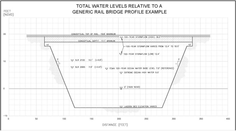
7.5.2 Highway 101 Bridges
Highway 101 bridge designs are the responsibility of local agencies. The information presented below is potential guidance for consideration by the local agencies for the design of these bridges. Most Highway 101 bridges cross lagoons over the tidal inlet and are adjacent to the coastline. These bridges are subject to both coastal and fluvial storm impacts. Therefore, the design for Highway 101 bridges should consider both fluvial and coastal processes. The bridge design should use the higher of design water levels determined in these two independent processes.
- The Fluvial Process: As discussed in Section 7.4 and shown on the right half of Figure 7-4, the design water level with SLR is determined by adding the SLR projection to the design ocean water level to form a new downstream boundary condition for the fluvial model runs. The final design water level under the 50- or 100-year storm event is determined through the use of fluvial hydraulic models that route river flows from upstream to downstream. Table 7-14 summarizes 50year and 100-year water levels, respectively, and the freeboard under the 100year storm for existing/current Highway 101 bridges from existing studies. Additional unsteady state numerical modeling studies for bridge design may need to be performed to fill data gaps and to yield consistent results. If no new modeling occurs, then the user can use existing stormflow elevations and add the SLR contributions between 2000 and 2030, 2050, and 2100 (a conservative approach).
- The Coastal Process: As shown in the left half of Figure 7-4 the final design water level of the coastal process is the wave crest elevation of the design wave while considering the projected SLR and wave setup in the design water depth. The design wave height is most likely depth-limited and the water depth at each Highway 101 bridge crossing is different; therefore, the design wave height needs to be calculated for each Highway 101 bridge. The wave set up is elevated water alongshore from high waves and depends on the design wave condition and beach slope. The wave setup also needs to be determined for each bridge.
The water level(s) to be used for the design of Highway 101 Project bridge structures should take into consideration all the information presented above, as summarized in Table 7-16 for each lagoon/river/creek.
Although the guidance provided above for tsunamis did not recommend using the tsunami water levels for design, the information is provided in the table below for completeness. Caltrans design guidance for tsunamis is provided in a previous section of this report (Caltrans 2010). Tsunamis should be considered as isolated events due to their relatively infrequent occurrence and potential severity. Although planning for their occurrence is warranted, the construction costs of infrastructure elevated for possible high tsunami water elevations are excessive. Therefore, designs should consider other processes such as high flow velocities and lateral support for impact during tsunami drainage.
As none of these bridges are being permitted as part of the PWP, a site-specific risk assessment approach may be needed to address future conditions. This type of assessment is presented in Section 8 of this document and entails determining site-specific needs for freeboard, and weighing the risk involved with the temporary closure of the bridge to travel if the closure duration is only a few hours (less than 6). Assessing the impact of potential closures relative to environmental impacts and costs of elevating infrastructure above all the highest combined water levels can help engineers determine appropriate "compromise" bridge elevations.
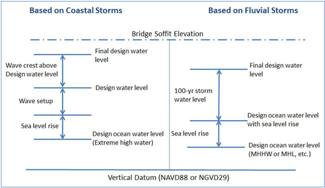
Table 7-16: Design Parameters for HW101 Project Bridges
| Design Parameters | Values | Unit / Datum |
|---|---|---|
| 100-year Extreme Ocean Water Level | 5.3 | feet / NGVD29 |
| SLR Increase w/Adaptation in Year 2100 | 1.5 | Feet |
| SLR Increase w/o Adaptation in Year 2100 | 3.0 | Feet |
| Observed Maximum Tsunami Wave Height | 1.5 | Feet |
| Fluvial Water Levels | Tables 7-13 and 7-14 | feet / NGVD29 |
| Design Wave Crest Elevation | TBD | feet / NGVD29 |
| Wave Setup | TBD | Feet |
7.5.3 Bridge Freeboards
Existing bridge freeboards were estimated using existing data for combined stormflows and existing and future sea-level conditions. Table 7-4 through Table 7-14 shows the freeboard for bridges on the railroad, I-5, and Highway 101 for water levels including up to 5.5 feet of sea-level rise. The tables show that under these conditions, six existing I-5 bridges may have freeboard issues in 2100 without replacement, while eight existing railroad bridges and seven existing Highway 101 bridges may have freeboard to be addressed.
8.0 Adaptive Management Strategy
Planning for SLR is a significant challenge due to the uncertainty of future SLR projections. Approaches can vary from "do nothing," to full preparation for the worst possible case, with multiple options between these extremes. Extreme approaches may or may not prove to be the most cost-effective solutions. The "do nothing" approach ignores the reality of SLR throughout the 20th Century along California and could prove problematic if even moderate SLR projections eventually occur. Conversely, full preparation for the worst possible scenario, which may never occur, may cause unnecessary environmental impacts to wetlands and exceed available project budgets. A more moderate and flexible approach can be taken that provides agencies with opportunities to proactively plan in a cost-effective manner.
The main recommended approaches are listed below:
- when feasible, design for the full range of sea levels for the life of the bridge structure;
- where not feasible due to some type of limitation (e.g., environmental, economic, social, etc.), design to the highest water level feasible and incorporate appropriate adaptive management strategies to enable raising infrastructure in the future; and
- site-specific analysis of conditions to set bridge elevations appropriately, given local conditions, potential environmental impacts and costs of higher bridges, and the risks posed by closing bridges for several hours infrequently due to a short-term fluvial event.
During the alternatives analysis phase, the full range of projected SLR scenarios should be considered and, if possible, the NCC Program projects should be designed to accommodate the high SLR projection of 5.5 feet between 2000 and 2100. If conflicting design requirements, like adjacent overhead bridges or impacts to sensitive wetlands, pose a project constraint limiting the PDT from designing to this projection, then adaptation strategies need to be considered.
Where adaptation strategies need to be considered for bridges, pre-cast structures are preferred over cast-in-place structures that cannot be raised in the future. More adaptive management approaches are provided below to implement changes incrementally in anticipation of progressively increasing water levels. The suggestions below could be implemented together to increase effectiveness.
8.1 Elevate New Infrastructure for Higher Sea Level Rise Scenarios
As aging infrastructure is gradually phased out and replaced with new construction, the new projects should be elevated to consider future higher water levels. Planning for high water levels is prudent during this period of high uncertainty. The appropriate high water level will vary from site to site, but common high water level conditions exist between sites that can be used in the estimate. Determination of the relatively higher probability high water levels for a particular location will require work by the implementing agency.
Designs should consider modeling results based on the ocean elevation of spring MHHW with the addition of the SLR projection of 5.5 feet between 2000 and 2100 using the NRC study, for a combined downstream high water level for flood modeling.
For Interstate 5 and NCC bridges, the final component of the high water level is stormflow. As this component is unique to each site, it needs to be estimated using a suitable approach. This fluvial value ranges depending on the site considered and the modeling approach used. This study recommends considering modeling of the 100-year flood with an unsteady state model, combined with a high downstream water level specified above. However, a more simplified and conservative approach is to use existing stormflow elevation predictions by Caltrans and others and adding 5.5 feet for SLR in 2100 on top of the model result. This resulting elevation could serve as the target bridge soffit elevation at a minimum. If FEMA requires additional freeboard, then that value should also be added.
Due to their proximity to the coastline, the final component of the high water level for Highway 101 bridges can be either the elevation of
- 100-year stormflow, or
- the elevation of the design wave crest plus wave set-up under future sea-level conditions. Therefore, the project design for Highway 101 bridges needs to consider both fluvial and coastal processes. The higher design water level determined in these two independent processes should be used as the final bridge design water level. To determine the design water level (wave crest plus wave set-up elevation) of the coastal process, the design wave height and wave setup need to be calculated for each bridge, and the appropriate SLR value (e.g., 5.5 feet at 2100) should be considered in the calculations of the design wave height and wave setup.
8.2 Install Adaptable Bridges and Approaches
Adaptive management of infrastructure is a likely requirement to address SLR. One possible adaptive management strategy is to design bridge structures and approaches now that can be raised in the future. Adapting the bridge structures and approaches to incrementally higher water levels over time may be less costly and less impacting to the environment than completely replacing bridges and raising approaches. A rough generic concept of an adaptable bridge structure is provided in Figure 8-1 and Figure 8-2. The concept can be applied to different bridge locations at the LOSSAN railway. Interstate 5 is sufficiently high to not need this approach.
The concept shows a pre-cast bridge with a larger foundation than would be required for existing conditions and bridge elevations. The larger foundation would serve to support the short-term bridge structure, as well as being capable of supporting a higher bridge structure if it needed to be elevated due to future SLR.
The LOSSAN corridor is planned for double-tracking. Figure 8-2 shows a single track bridge, assuming the second track of a double-track bridge is carried by a parallel bridge; however, the concept would also work with a wider double-track bridge. The bridge and approaches would be constructed at the appropriate elevation for design conditions, and then raised in the future to accommodate changed sea-level conditions as needed. The sketch shows an increase in elevation of approximately five feet, similar to the high projection of SLR in the year 2100 (5.5 feet).
General features that would help facilitate raising the bridge at a future time are listed below.
- Simple span precast box beams (this is a standard BNSF/UPRR bridge type for LOSSAN);
- Bearing pads under the box beams so that beams are not permanently connected to the substructure;
- Oversized end diaphragms of the box beams to allow space to jack the bridge;
- Substructure (piers, abutments, foundations) designed for the final raised condition;
- Pier walls (if not a pile structure) that readily accommodate an increase in elevation on the order of five feet;
- Pile caps that extend beyond the face of the pier wall to make it easy to jack the bridge utilizing the bridge's foundations forbearing. No temporary piling would be required (driving temporary piles under the completed bridge would be difficult);
- Pile caps designed to support the future jacking loads; and
- Widened earthen berms at bridge approach during initial construction to allow for raising of the berms in the future to support a higher rail line to meet the raised rail bridges. The design of widened berms needs to be done in consideration of site-specific conditions.
Jacking up of the rail bridge, as shown in Figure 8-2, would be done incrementally with shims inserted between a series of smaller-scale vertical motions of the bridge.
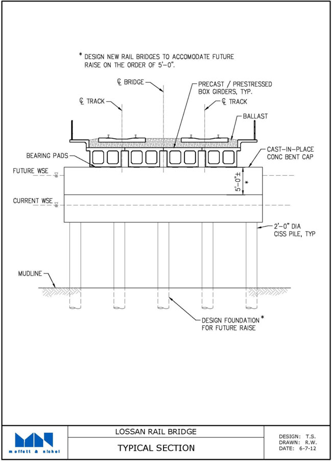
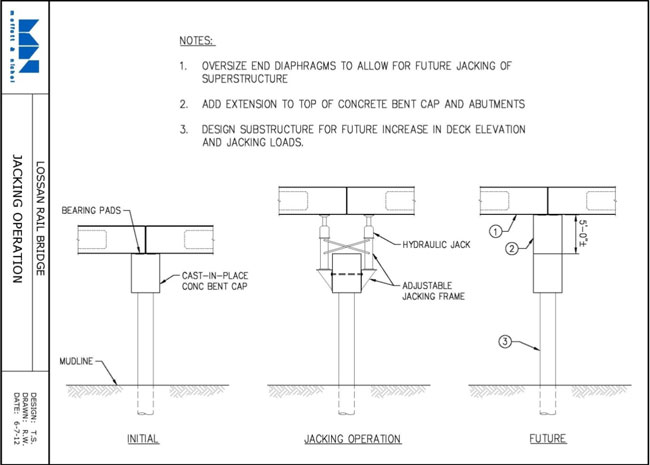
Utilizing a movable bridge concept in combination with elevating new infrastructure should provide the PDT with sufficient latitude to implement projects that can change over time more cost-effectively than total replacements. It allows for the structures to remain in use throughout their typical lifespans for maximum utility and provides additional time for the PDT to gather new information about future high water levels for future projects.
8.3 Estimate Conservatively High Water Levels and Raise New Bridges on I-5
A conservative method to calculate high water levels under I-5 bridges would be to add 5.5 feet of SLR in 2100 to the predicted 100-yr design stormflow water elevations for existing sea-level conditions. New bridges to be installed on I-5 could be elevated to sufficiently clear this condition, plus any required freeboard value of FEMA. Several bridges need to be addressed and may require design features to consider higher water levels.
8.4 Estimate New and Less Conservative High Water Levels and Raise New Bridges on I-5 – Conduct a Site-Specific
If I-5 bridge elevations would be too high from the previous approach and not considered feasible for appropriate reasons, then re-model the sites using the same methods as those employed in the bridge optimization studies by Caltrans (EIC 2011, M&N 2012a and 2012b). These new elevation values would then be the new design basis for bridge designs. New bridges to be installed on I-5 could be elevated to clear this condition, plus any required freeboard value of FEMA. New modeling with an unsteady state model would potentially yield lower water levels than the simple addition of SLR (e.g., 5.5 feet by 2100) to the 100-year flood elevation because of effects on lagoon geometry on hydraulics.
8.5 Conduct a Site-Specific Design Water Level Analysis Methodology Considering Sea Level Rise
A site-specific analysis approach is presented below that can be used to help guide future design efforts for bridges and embankments located within the NCC. The steps summarized below would be completed to establish the future mean sea level range to be considered in the development of design water levels for the bridge and embankment structures.
- Establish a range of future regional/local relative mean sea level change projections that is consistent with the latest scientific information on regional/local sea level, and land subsidence and uplift. This can be done by either updating this San Diego Region Coastal Sea Level Analysis Report to the current scientific estimates, or following the steps listed below:
- a. Review the latest scientific literature on global/regional mean sea level rise to identify the most relevant scientific information for the project area.
- b. Review the latest governmental guidance related to global/regional mean sea level rise from federal, state, and local agencies with regulatory responsibilities for the project.
- c. Establish a range of future global/regional mean sea level rise projections that is consistent with the most relevant scientific information and governmental agency guidance from Steps a and b above, respectively.
- d. Review the latest scientific literature on regional/local land subsidence and uplift to better assess how to land elevations relative to sea level elevations that may change over the life of the project.
- For bridges and embankments located far enough from the ocean such that ocean waves do not directly impact structures, the high water level to be used for design is controlled by the fluvial process. The high water level can be established by conducting fluvial hydraulic modeling using design storm events (e.g., 50-year and 100-year flows) at the upstream boundary and a high water level at the downstream boundary (e.g., MHHW or the 50-year ocean water level, or following design guidelines by Caltrans or Railroad agencies) which would either be the ocean or lagoon. This step should be repeated across the range of future regional/local, relative mean sea level change projections established under Step 1 above. This could be done by analyzing only the design condition if the only issue of concern for design is the design water level or it could entail analyzing the highest and lowest condition to bracket the full range of potential water levels that the project may experience in the future under higher mean sea level conditions. It might even be helpful to analyze intermediate conditions if such information would be useful for conducting optimization analyses for such issues as potential environmental impacts and economic considerations (e.g., Step 4 below).
- For bridges and embankments located close enough to the ocean such that ocean waves may directly impact structures, the high water level to be used for design may need to be based on both fluvial or coastal processes. These structures are subject to both coastal and fluvial storm impacts and, therefore, the project design needs to consider both fluvial and coastal processes. The bridge design should use the higher of design water levels determined in these two independent processes.
- a. The Fluvial Process: Use procedures described in Step 2 above to determine the design water level under the fluvial process.
- b. The Coastal Process: The high design water level should include contributions from the astronomical tide, barometric pressure, wave crest elevation, wave set-up, El Nino Southern Oscillation (ENSO), and Pacific Decadal Oscillation (PDO). Depending on the situation, wave run-up on the structure (e.g., embankment) may also need to be considered in establishing the extreme high ocean water level. This step should be repeated across the range of future regional/local, relative mean sea level change projections established under Step 1 above. This could be done by analyzing only the design conditions if the only issue of concern for design is the design water level, or it could entail analyzing the highest and lowest condition to bracket the full range of potential water levels that the project may experience in the future under higher mean sea level conditions. It might even be helpful to analyze intermediate conditions if such information would be useful for conducting optimization analyses for such issues as potential environmental impacts and economic considerations (e.g., cost-benefit analysis).
- Conduct analyses to evaluate trade-offs related to bridge and embankment design. This would include consideration of environmental impacts (e.g., visual and habitat impacts), constructability, construction and maintenance costs, and economic (e.g., cost-benefit) considerations. In addition, a risk assessment should be performed to determine the consequences of failing to address sea-level rise adequately for a particular project and the potential impacts on public health and safety, public investments, and the environment. For example, the risk assessment could evaluate the consequences to fully accommodate the combined "worst possible case" scenario of the highest sea-level rise condition in combination with a 100-year river or stream flood event. The actual duration of freeboard exceedance at bridges during such an event is likely to be very short. For example, the duration of the freeboard exceedance of 0.5 feet at the proposed I-5 bridge over Batiquitos Lagoon shown in Table 7-11 is 2 hours (M&N 2012a). This approach may not be feasible due to the potential for permanent environmental impacts to wetlands caused by the construction of a project to prevent a very short duration bridge closure. At this step, the PDT would have to decide whether to:
- design a structure such that it is above the highest future projected water level;
- design a structure such that it is above a lower future projected water level but allows for adaptive strategies to address higher future projected water levels; or
- establish a design water surface elevation for use based on this risk assessment.
8.6 Periodically Update Design Guidelines for High Water Levels
These design guidelines for high water levels should be periodically updated to incorporate new information as it becomes available and as local conditions change. The guidelines should reconsider all high water level values so that changes to any components can be made if climate change occurs and sufficient data are available for analyses. Climate change may cause variations in each component, except for tsunamis. The frequency of updating design guidelines may need to be every 10 years initially, and then modified after that depending on existing trends of high water levels components, updated SLR predictions of the future, and probabilities (once available) associated with SLR predictions.
A combined approach of all of the above-mentioned adaptation strategies may serve the PDT's best and provide the greatest degree of flexibility. Additional adaptation strategies could be added to this list, as appropriate, when the design guidelines are updated. The broadest range of possible actions will give SANDAG and Caltrans the greatest suite of tools to apply to this complex challenge.
9.0 General Conclusions and Recommendations
The NCC Program requires planning and engineering of coastal rail and highway infrastructure to potential future high water levels as a result of SLR. SLR represents a significant variable influencing the NCC Program highway and rail bridge design as well as the future success of the Program. Data are presented to show bridge soffit elevations for the railroad, I-5, and Highway 101 under high water scenarios combined with future sea-level rise. Multiple bridges in each transportation corridor show concerns relative to elevation versus combined high water in the future.
The following recommendations are offered for the consideration of SLR in the design of the individual components of the Program:
- PDTs should consider the full range of SLR projections in the alternatives analysis phase for the design life of various projects under the Program (75 years plus 10 years, assuming proper maintenance). Based on the results of the alternatives analysis, the preliminary design either will: 1) accommodate the maximum SLR projection of 5.5 feet by 2100; 2) be designed with adaptation strategies and an SLR rate that is as high as can be accommodated; or 3) be designed according to the site-specific analysis of local conditions and needs, environmental impacts, and risks involved with closing bridges for very short periods i]on an infrequent basis. Adaptive strategies would allow bridge structures and approaches to be raised in the future should the projections occur.
- Since the Program has the potential to receive funding from both state and federal sources, it is recommended that it be consistent with the most recent guidance from both of these sources.
- a. Consider a range of SLR projections in the years 2050 and 2100 to satisfy State guidance from 2013. It is recommended that SLR projections from State guidelines be applied to fulfill this requirement. At 2050, the maximum SLR projection is 2 feet, and at 2100, the SLR projection is 5.5 feet.
- b. For the LOSSAN railroad and Interstate 5 bridges, the PDTs should consider SLR scenarios in combination with 50-year and 100-year storm flow events since these events are higher than extreme ocean high water events (e.g., high tides and storm surge). The 100-year stormflows from North County coastal streams result in water levels that increase significantly above the extreme tide. Existing stormflow modeling results should be used with a value of 5.5 feet for SLR in 2100 to provide conservative high water values for planning and design. Detailed modeling with an unsteady state model could be done to produce more accurate and consistent values if appropriate. Several coastal streams have been recently modeled to determine accurate and more comparable water levels during high floodwaters. Other Lagoon and/or Creeks would need to be modeled with an approach similar to the approach used in the bridge optimization studies conducted for Caltrans to determine their respective more comparable high floodwater levels.
- Highway 101 bridges warrant site-specific analyses to identify the condition of the highest combined water levels, and design guidelines need to be developed. Due to their proximity to the coastline, both the 100-year fluvial storm flood level and extreme wave crest and set-up elevation need to be calculated for each bridge since they are unique to each bridge. The higher design water level determined in these two independent processes should be used as the final bridge design water level. For the fluvial storm flood levels, the same approach as indicated above should be applied. New site-specific modeling could be done with an unsteady state model to produce more accurate and consistent results with other studies. Several coastal streams have been recently modeled to determine accurate and comparable water levels during high floodwaters. Other lagoons and creeks would need to be modeled with an approach similar to the approach used in the bridge optimization studies conducted for Caltrans as indicated above to determine their respective and comparable high floodwater levels. All such work for Highway 101 bridges would be done by local agencies. Improving the hydraulic conveyance conditions of Highway 101 bridges would likely lower water levels upstream at rail and I-5 bridges during 100-year floods.
- Tsunamis have the potential to impact the study area. Based on the observed data, the study area could be impacted by a tsunami with a maximum wave height of approximately 3 feet every ten years. This wave will diminish in height as it propagates into a lagoon and would likely be below the elevation of the 100-year stormflow, so its height is not the primary design concern. The concern from a tsunami is the increase in flow velocities under bridges from high current velocities. Consequently, bridges should be designed with additional scour protection on both sides of the bridge abutments and be supported on piles/piers to resist erosion associated with the high water velocities that are expected to occur during tsunamis. A secondary concern may be lateral forces exerted by any impact, and potential uplift, requiring bolting to the foundation. Bridge design should consider additional lateral support and uplift to resist tsunamis, should they occur.
- SANDAG should review upcoming updates to California and Federal guidance to continually update bridge design guidance. Upcoming guidance of interest includes the following:
- a. IPCC Fifth Assessment Report (due in 2013);
- b. U.S. Climate Change Science Program Synthesis and Assessment Studies; and
- c. FEMA National Climate Change Study.
- Since the magnitude of SLR is highly uncertain, an adaptive management approach should be adopted toward the development of new infrastructure within the region. This approach may include:
- a. Design new structures to be high enough to accommodate the high SLR scenarios offered by the State and Federal guidelines, if feasible. The latest higher limit projection by the NRC is 5.5 feet in 2100.
- b. For railroad bridges, if it is not feasible to accommodate high SLR projections, incorporate adaptable components into railroad bridge designs to enable jacking of the structures upward and raising approaches to accommodate future higher water level conditions, should they occur. Foundations can be designed to allow adaptation of the bridge and approaches in the future. Railroad bridge approaches should be designed to allow a sufficient footprint for increasing the elevation and width of berms to match elevated bridges. Incorporation of this design feature may be less costly and less impacting than bridge replacement in the future if elevated water levels occur. This approach enables the PDT to make maximum use of new bridges and provides additional time to consider water level data in the future.
- c. For I-5 bridges, strategies could be to evaluate bridges in more detail when their replacement date arrives and use an unsteady state model to better understand water levels. Also, bridges may be able to experience high water in contact with the structure for a short duration (during the peak of the flood in future SLR conditions) while remaining open to traffic if the travel lanes remain dry. Finally, certain less critical bridges (e.g., bicycle bridge in Los Peñasquitos Lagoon) may need to be temporarily closed during such an event.
- d. For all bridges, conduct site-specific design water level analysis considering sea-level rise to set the appropriate design water level at each bridge when needed. The analysis would focus on identifying the dominant process causing high water levels at each bridge, the resulting water surface elevation, and risk assessment of construction to accommodate the high water level projection. The risk assessment would consider the level of protection versus costs, impacts, and duration of bridge closures, considering the probability of occurrence.
- e. Update water level guidance documents as new sea-level rise projections are made available from progressing science and/or guidance.
- f. For bridges that may not meet water level guidelines, consider site-specific analyses for the Public Works Plan document such as:
- i. As indicated previously, updating modeling to generate more accurate and consistent results with unsteady-state models, and consider results in designs.
- ii. Comparing water levels with criteria other than bridge soffits, such as the ballast for the railroad and travel lanes for I-5, and plan management actions according to engineering judgment; actions could include closing bridges for the period (as mentioned above) when water levels exceed elevations of rail ballast or I-5 travel lanes, respectively, and reopen the bridges when water levels drop below these thresholds.
10.0 References
- American Railway Engineering and Maintenance-of-Way Association (AREMA). 2009. Manual for Railway Engineering. Volume 1. Track. 2009.
- Ballona Wetlands Land Trust v. City of Los Angeles (Case No. B231965)
- Abbott, Patrick L. 1999. The Rise and Fall of San Diego. 150 Million Years of History Recorded in Sedimentary Rocks. Sunbelt Publications, Inc. 1999.
- BBC. 2012. Composition of the Earth's Atmosphere. January 2012.
- Bromirski, P.D., A.J. Miller, R.E. Flick, and G. Auad. 2011. Dynamical Suppression of Coastal Sea Level Rise. Unpublished Draft Submitted to the Journal of Geophysical Research. January 2011.
- California Coastal Commission. 2001. Overview of Sea Level Rise and Some Implications for Coastal California. Miscellaneous Report.
- California Natural Resources Agency. 2009. Executive Summary, 2009 California Climate Adaptation Strategy, First Year Progress Report to the Governor of the State of California in Response to Executive Order S-13-2008. August 23, 2009.
- 2010. 2009 California Climate Adaptation Strategy, First Year Progress Report to the Governor of the State of California.
- California State Coastal Conservancy (CSCC). 2009. Coastal Conservancy Climate Change Policy and Project Selection Criteria. Adopted June 4, 2009.
- Caltrans. 2010. Memo to Designers 20-13. Tsunami Hazard Guidelines. January 2013.
- 2011. Guidance on Incorporating Sea-level Rise. Prepared by the Caltrans Climate Change Workgroup and the HQ Divisions of Transportation Planning, Design, and Environmental Analysis. May 16, 2011.
- 2012. A table titled "Bridge 100-year Flood Freeboard for Interstate 5," provided by Caltrans to RailPros staff.
- 2013. Interstate 5 North Coast Corridor Project. Draft Public Works Plan/Transportation and Resource Enhancement Program. March 2013.
- Cayan, D., et al. 2009. Sea Level Rise Estimates for the California 2008 Climate Change Scenarios Assessment. California Climate Change Center, CEC-5002009-014-F.
- Cazenave, A., A. Lombard, and W. Llovel. 2008. Present-Day Sea Level Rise: A Synthesis. Comptes Rendus. Geoscience 340, pp. 761-770.
- CCCC. 2006. Projecting Future Sea-level. California Climate Change Center. California Energy Commission, Public Interest Research Program. CEC-500-2005-202-SF. March 2006.
- 2009a. Climate Change Scenarios and Sea-level Rise Estimates for the California 2008 Climate Change Scenarios Assessment, Draft Paper. California Climate Change Center. California Energy Commission, Public Interest Research Program. CEC-500-2009-014-F. March 2009.
- 2009b. Climate Change Scenarios and Sea-level Rise Estimates for the California 2009 Climate Change Scenarios Assessment, Final Paper. California Climate Change Center. California Energy Commission, Public Interest Research Program. CEC-500-2009-014-F. August 2009.
- 2009c. The Impacts of Sea-level Rise on the California Coast. California Climate Change Center. Prepared for the California Energy Commission, Public Interest Research Program. CEC-500-2009-024-F. May 2009.
- Centre National d'Etudes Spatiales (CNES) and Collecte Localisation Satellites (CLS). 2010. AVISO: Mean Sea Level Rise. http://www.aviso.oceanobs.com/en/ news/ocean-indicators/mean-sea-level/.
- Chang. H.H. 2010. Hydraulic and Scour Studies for Proposed Interstate-5 Bridge Widening Across Three Lagoons. Chang Consultants. July 2010.
- Chao, B.F., Y.H. Wu, and Y.S. Li. 2008. Impact of Artificial Reservoir Water
- Impoundment on Global Sea Level. Science Magazine 320, pp. 212-214.
- Clough, Jonathan S., and Evan C. Larson. 2009. Warren Pinnacle Consulting, Inc. Application of SLAMM 5.1 to San Diego County, CA. Prepared for Dr. Rick Gersberg; San Diego State University.
- Centre National d'Etudes Spatiales (CNES) and Collecte Localisation Satellites (CLS). 2010. AVISO: Mean Sea Level Rise. http://www.aviso.oceanobs.com/en/ news/ocean-indicators/mean-sea-level/
- Coastal Environments. 2010. San Dieguito Lagoon Restoration Project: Historical Beach Data Adjacent to San Dieguito Lagoon. A report in Partial Satisfaction of Coastal Commission Permit Number 6-04-088. December 30, 2010.
- CO-CAT. 2010. State of California Sea-Level Rise Interim Guidance Document. Sea-Level Rise Task Force of the Coastal and Ocean Working Group of the California Climate Action Team. October 2010.
- CO-CAT. 2013. State of California Sea-Level Rise Guidance Document. Coastal and Ocean Working Group of the California Climate Action Team. March 2013 Update.
- Douglass, Scott L, and Joe Krolak. 2008. Highways in the Coastal Environment, Hydraulic Engineering Circular 25, Second Edition. Report No. FHWA NHI-07096. U.S. Department of Transportation Federal Highway Administration. June 2008.
- David Dykstra. 2012. Supervisory Coastal Engineer. Moffatt & Nichol. Personal Communication With Chris Webb on January 24, 2012.
- Encyclopedia Britannica Online. 2012. Air (atmospheric Gas). Encyclopedia Britannica,
- n.d. Web accessed on 11/30/12. http://www.britannica.com/EBchecked/topic/10582/air.
- Everest International Consultants (EIC). 2004. Buena Vista Lagoon Restoration Feasibility Analysis. Final Report. Volume 1. Main Report. June 2004.
- 2009. Approach to Incorporate Projected Future Sea Level Change into the Encinitas & Solana Beach Shoreline Protection Feasibility Study and CEQA and NEPA Compliance Efforts. A memo prepared for the USACE-SPL, by the Cities of Encinitas and Solana Beach with assistance from EIC and EDAW.
- 2011. Draft Sea-Level Rise Report for the San Luis Rey Bridge Replacement. Prepared for HNTB Corporation. December 2011.
- 2011. Bridge Optimization Study for Buena Vista Lagoon. December 2011.
- Federal Emergency Management Agency. 1991. Projected Impact of Relative Sea-level
- Rise on the National Flood Insurance Program. Federal Emergency Management Agency, Federal Insurance Administration. October 1991.
- 2000. Evaluation of Erosion Hazards. Prepared by The H. John Heinz III Center for Science, Economics, and the Environment. Prepared for the Federal Emergency Management Agency. April 2000.
- 2004. Guidelines and Specification for Flood Hazard Mapping Partners. Various documents available from FEMA and the Department of Homeland Security at http://www.fema.gov/plan/prevent/fhm/gs_main.shtm#6
- 2005. Final Draft Guidelines for Coastal Flood Hazard Analysis and Mapping for the Pacific Coast of the United States. Prepared for the Federal Emergency Management Agency. Revised January 2005.
- 2010. Impact of Climate Change on the NFIP. Presentation to the Coastal Engineering Research Board Meeting June 22, 2010, by Mark Crowell.
- 2011a. Coastal Construction Manual, Principles and Practices of Planning, Siting, Designing, Constructing, and Maintaining Residential Buildings in Coastal Areas (Fourth Edition). FEMA P-55 / Volume I & Volume II / August 2011.
- 2011b. Strategic Plan Evaluation Climate Change and the Community Rating System. National Flood Insurance Program Community Rating System. June 2011.
- Governor of the State of California. 2005. Executive Order S-3-05. Office of the Governor of the State of California, Governor Arnold Schwarzenegger. June 1, 2005.
- 2008. Executive Order S-13-08. Office of the Governor of the State of California, Governor Arnold Schwarzenegger. November 14, 2008.
- Flick, R.E., J.F. Murray and L.C. Ewing. 2003. Trends in United States Tidal Datum Statistics and Tide Range, J. Waterway, Port, Coastal and Ocean Engineering. American Society of Civil Engineering. 129 (4), 155-164.
- Griggs, Gary. 2012. Presentation to the American Shore & Beach Preservation Association, Annual 2012 Conference, San Diego, CA. October 11, 2012.
- Hanson-Wilson, Inc. 2004. NCTD Bridge 230.6 Hydrology/Hydraulics Report, pg 3. July 2004.
- Heberger, M., et.al. 2009. The Impacts of Sea Level Rise on the California Coast. California Climate Change Center, CEC-500-2009-024-D.
- HDR. 2008. Final Drainage and Scour Analysis, page 9-10. May 2008.
- 2009a. Final Drainage and Scour Analysis Technical Memorandum, Bridge 240.4, San Elijo Lagoon. January 2009.
- 2009b. Final Drainage and Scour Analysis, Bridge 246.1. February 2009.
- 2009c. Final Drainage and Scour Analysis, Bridge 246.9. February 2009.
- 2009d. Final Drainage and Scour Analysis, Bridge 247.1. February 2009.
- 2010a. Draft Sorrento Valley Double Track Drainage Report, pg. 19. May 2010.
- 2010b. Draft Drainage Report, Bridge 249.9. September 2010.
- 2011. Draft Sorrento Valley Double Track Drainage Report, Bridge 247.7, Model Update, June 2011.
- 2011a. Hydraulic and Scour Analyses Technical Memorandum (DRAFT), Bridge 240.0. December 2011.
- HNTB. May 2012. Final Hydrology and Hydraulics Report for East Brook to Shell Double Track Project, Prepared for SANDAG.
- Houston, J.R. and R.G. Dean. 2011. Sea-Level Acceleration Based on U.S. Tide Gauges and Extensions of Previous Global-Gauge Analyses. May 2011.
- IBI Group. 2009. Conformed Plans, Sheet s-03. October 2009.
- International Council for Local Environmental Initiatives – Local Governments for Sustainability USA (ICLEI). 2012. Sea Level Rise Adaptation Strategy for San Diego Bay. January.
- Intergovernmental Panel on Climate Change (IPCC). 2001. Climate Change 2001: The Scientific Basis. Contribution of Working Group I to the Third Assessment Report of the Intergovernmental Panel on Climate Change. Houghton, J.T., Y. Ding, D.J. Griggs, M. Noguer, P.J. van der Linden, X. Dai, K. Maskell, and C.A. Johnson (eds.), Cambridge University Press. Also available online at <http://www.ipcc.ch/>.
- 2007. Climate Change 2007: The Physical Science Basis. Contribution of Working Group I to the Fourth Assessment Report of the Intergovernmental Panel on Climate Change. Solomon S., D. Qin, M. Manning, Z. Chen, M. Marquis, K.B. Averyt, M. Tignor, and H.L. Miller (eds.), Cambridge University Press. Also available online at http://www.ipcc.ch/.
- Jet Propulsion Laboratory (JPL). October 2012. Could a Hurricane Ever Strike Southern California? http://www.jpl.nasa.gov/news/news.php?release=2012-329.
- Messner, S., C. Phillips, D. Cayan, and E. Young. 2008. The San Diego Foundation Regional Focus 2050 Study. Climate Change Related Impacts in the San Diego
- Region by 2050. Working Papers for the 2008 Climate Change Impacts Assessment, Second Biennial Science Report to the California Climate Action Team.
- LaHood, Ray. 2011. Policy Statement on Climate Change Adaptation. United States Department of Transportation.
- Messner, S., C. Phillips, D. Cayan, and E. Young. 2008. The San Diego Foundation Regional Focus 2050 Study. Climate Change Related Impacts in the San Diego
- Region by 2050. Working Papers for the 2008 Climate Change Impacts Assessment, Second Biennial Science Report to the California Climate Action Team.
- Moffatt & Nichol. 2010. San Elijo Lagoon Restoration Project Sea Level Rise Analysis. Draft Report. Prepared for the San Elijo Lagoon Conservancy.
- 2011. San Dieguito Lagoon Project. Hydrology/Hydraulic Study. Final Report. December 2011.
- 2012. San Elijo Restoration Project Hydrology/Hydraulic Study. Final Report. Prepared for the San Elijo Lagoon Conservancy. June 2012.
- 2012a. Batiquitos Lagoon Bridge Optimization Study. Final Report. April 2012.
- 2012b. San Elijo Lagoon Bridge Optimization Study. Final Report. Prepared for the San Elijo Lagoon Conservancy. April 2012.
- National Geographic. 2012. http://ocean.nationalgeographic.com/ocean/critical-issuessea-temperature-rise/.
- National Research Council of the National Academy of Sciences (NRC). 1987. Responding to Changes in Sea-level: Engineering Implications. Committee on Engineering Implications of Changes in Relative Mean Sea-level; Marine Board, Commission on Engineering and Technical Systems, National Research Council. National Academy Press. Washington, D.C. in 1987.
- 2012. Sea-Level Rise for the Coasts of California, Oregon, and Washington: Past, Present, and Future. The National Academies Press. 2012.
- NIPP. 2009. National Infrastructure Protection Plan, Partnering to enhance protection and resiliency.
- NOAA Tides & Currents. 2012. Mean Sea Level Trend – 9410230 La Jolla, California. Viewed online at http://tidesandcurrents.noaa.gov/sltrends/. January 17, 2012.
- 2012a. Mean Sea Level Trend – San Diego, California. Viewed online at: http://tidesandcurrents.noaa.gov/sltrends/. January 17, 2012.
- 2012b. Extreme Water Levels, 9410230 La Jolla, California. http://tidesandcurrents.noaa.gov/est/stickdiagram.shtml?stnid=9410230.
- OPC (California Ocean Protection Council). 2011. Resolution of the California Ocean Protection Council on Sea-level Rise. March 11, 2011.
- Rahmstorf, S. 2007. A Semi-Empirical Approach to Projecting Future Sea-Level Rise. Science Magazine 315, pp. 368-370.
- Rick Engineering. 2010. Loma Creek LOMR Application. Prepared for SPRINTER Rail Project. January 2010.
- Richter, James, AMTRAK, Deputy Chief Engineer-Structures. Personal Communication April 5, 2012.
- SANDAG. 2009. San Diego – LOSSAN Corridor Project Prioritization Analysis. July 2009.
- 2010a. Climate Action Strategy. March 2010.
- 2011. 2050 Regional Transportation Plan. October 2011.
- Smith, Bruce. 2012a. Personal Communication with Chris Webb of Moffatt & Nichol on January 9, 2012.
- Southern California Edison (SCE). 2011. Southern California Edison's Evaluation of California Energy Commission AB 1632 Report Recommendations, Appendix 2 "Tsunami Hazard Evaluation". February 2011.
- The state of California. 2009. Tsunami Inundation Map for Emergency Planning, San Diego County; produced by California Emergency Management Agency, California Geological Survey, and University of Southern California – Tsunami Research Center; mapped at 1:24,000 scale. 2009.
- Steffensmeier, Chuck. 2013. Senior Transportation Engineer, San Diego Association of Governments. Personal Communication with Chris Webb on January 21, 2013.
- USACE. (U.S. Army Corps of Engineers). 2002. Coast of California Storm and Tidal Waves Study, South Coast Region, Orange County. USACE, Los Angeles District. December 2002.
- 2009a. Water Resource Policies and Authorities Incorporating Sea-level Change Considerations in Civil Works Programs. Department of the Army, U.S. Army Corps of Engineers, Washington, DC, Engineer Circular (No.1165-2-211). July 1, 2009.
- 2009b. Policies for Referencing Project Elevation Grades to Nationwide Vertical Datums. U.S. Army Corps of Engineers. ER 1110-2-8160. March 1, 2009.
- 2010. Standards and Procedures for Referencing Project Elevation Grades to Nationwide Vertical Datums. U.S. Army Corps of Engineers. EM 110-2-6056. December 31, 2010.
- 2011. Sea-level Change Considerations for Civil Works Programs. Department of the Army, U.S. Army Corps of Engineers. EC 1165-2-212. October 1, 2011.
- Vermeer, Martin, and Rahmstorf, Stefan. 2009. Global sea-level linked to global temperature. Proceedings of the National Academy of Sciences Early Edition, DOI: 10.1073/pnas.0907765106.
- 2011. Discussion of: Houston, J.R. and Dean, R.G., 2011. Sea-Level Acceleration Based on U.S. Tide Gauges and Extensions of Previous GlobalGauge Analysis. Journal of Coastal Research, 27(3), 409-417.
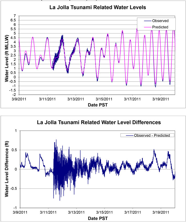
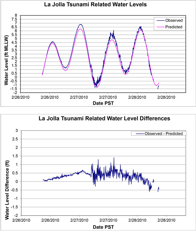


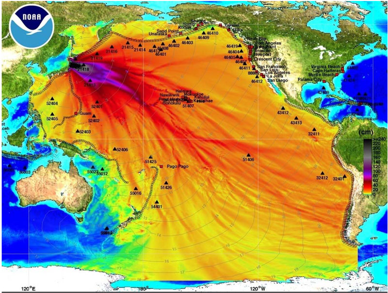
List of Acronyms
| 4AR | Fourth Assessment Report |
| Caltrans | California Department of Transportation |
| CAS | Climate Action Strategy (from SANDAG) |
| CCCC | California Climate Change Center |
| CCSM | Community Climate System Model (from NCAR) |
| CDIP | Coastal Data Information Program (at SIO) |
| CEQA | California Environmental Quality Act |
| CNRM | Centre National de Recherches Meteorologiques |
| CO-CAT | Coastal and Ocean Working Group of the California Climate Action Team |
| CSCC | California State Coastal Conservancy |
| EC | Engineering Circular |
| EIR | Environmental Impact Report |
| ENSO | El Niño Southern Oscillation |
| EO | Executive Order |
| FEMA | Federal Emergency Management Agency |
| FHWA | Federal Highway Administration |
| FRA | Federal Rail Authority |
| FTA | Federal Transit Authority |
| HEC | Hydraulic Engineering Circular |
| ICLEI | International Council for Local Environmental Initiatives |
| IPCC | Intergovernmental Panel on Climate Change |
| LOSSAN | Los Angeles to San Diego |
| MLLW | Mean Lower Low Water |
| MSL | Mean Sea Level |
| NAS | National Academy of Sciences |
| NAVD | North American Vertical Datum |
| NCAR | National Center for Atmospheric Research |
| NCC | North Coast Corridor |
| NRC | National Research Council |
| NEPA | National Environmental Protection Act |
| NFIP | National Flood Insurance Program |
| NGVD | National Geodetic Vertical Datum |
| NIPP | National Infrastructure Protection Plan |
| NOAA | National Oceanic and Atmospheric Administration |
| NRC | National Research Council |
| OPC | Ocean Protection Council |
| PDO | Pacific Decadal Oscillation |
| PDT | Project Development Team |
| PID | Project Initiation Document |
| PIER | Public Interest Energy Research |
| POLA/POLB | Ports of Los Angeles and Long Beach |
| SANDAG | San Diego Association of Governments |
| SCC | State Coastal Conservancy |
| SIO | Scripps Institution of Oceanography |
| SLC | State Lands Commission |
| SLR | Sea Level Rise |
| TAR | Third Assessment Report |
| USACE | U.S. Army Corps of Engineers |
| USDOT | U.S. Department of Transportation |